Named Ranges in Excel – Define, Usage, and Types

Named Ranges play a fundamental role in defining efficient and easy-to-read excel functions and formulas. It can also be used in Data Validation and hyperlinks.

Let us understand the concept.

What are Named Ranges in Excel?

The named ranges help give human-defined names to a particular cell reference, range, or group of ranges. It is a different way of naming our cell references which we can use in our formulas.

For Example:- Let us suppose we want to find the maximum value in the range A1:A291. We can use the MAX formula as

=MAX(A1:A291)

Or we can simply name the range A1:A291 as data and then simply use the “data” as the reference to rage A1:A291

=MAX(data)

Once we have created the named range “data”, it appears while writing this MAX formula as:-

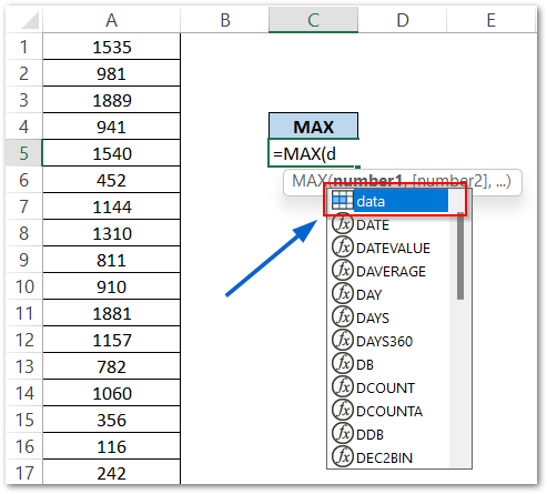
Here you can see that the “data” appears on top of the list while typing the formula. Hit the Tab key and then Enter key.

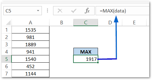
So you can see here that typing “data” is much easier than typing A1:A291. Also, it made our formula easier to read,

How to Create Named Ranges in Excel?

There are multiple ways to make a named range in excel. Let’s check them all.

Method 1 – Using the Name Box

This is the simplest way to name a range. All you need to do is:-

• Select the range of cells that you wish to name.
• Go to the Name Box and type the “marks” as the name of the range A2:A5.

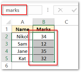
Now the “marks” specify the range B2:B5 in the formula. We can also use other formulas such as

=SUM(marks)

=AVERAGE(marks)

=MIN(marks)

Method 2- Using the Ribbon

To create a named range from this ribbon simply:-

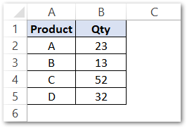
• Select the range B2:B5
• Go to the Formulas tab on the ribbon.
• Navigate to the Define Names Group and click on Define Name Button.

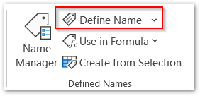
• In the New Name dialog box, fill the name field and then click ok.

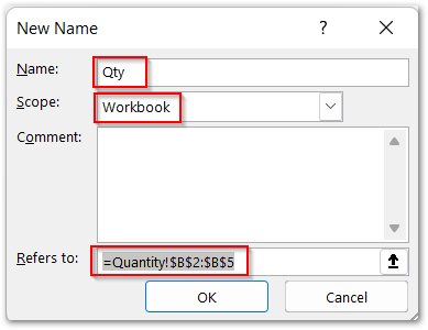
Here we have three fields:-

• Name:- specifies the name of the new named range.
• Scope:- specifies the scope where the named range would be considered valid. By default, it is set to the entire workbook.
• Refers to:- specifies the range at which the named range points. By default, named ranges use absolute referencing.

Method 3 – Using the Shortcut Ctrl+Shift+F3

Let us suppose we have the salaries of different employees of a company as follows:-

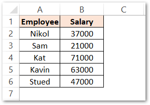
• Select the range A2:B6 and press the Ctrl Shift F3 key.

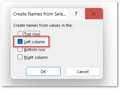
• As the Employee names are contained in the left column of the range A2:B6, mark the option for Left Column in the Create Names from Selection dialog box. Click Ok

How to see the Defined Named Ranges?

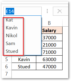
Now you can see that the references to employee salary will be named as employee name. You can see that in the Name Box Drop Down list.

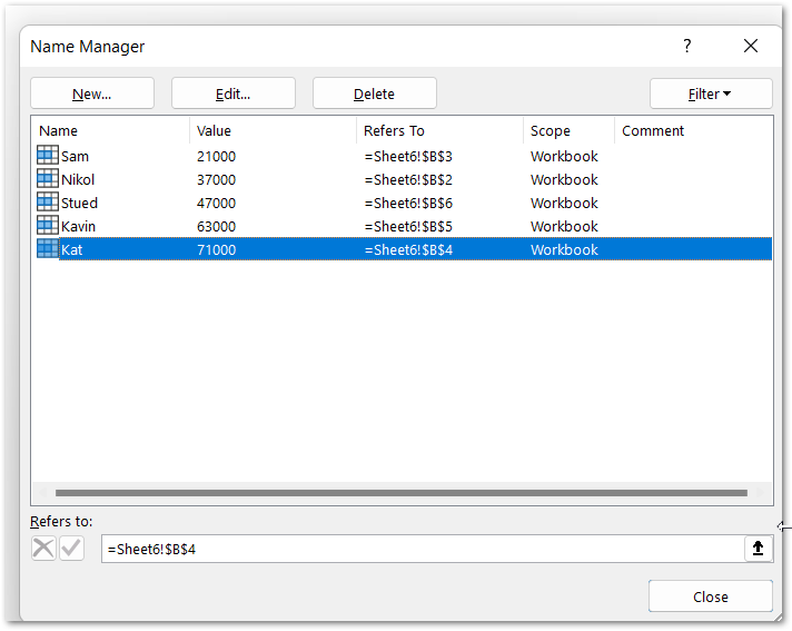
The shortcut to check all the named ranges is to press Ctrl F3 key. This opens the Name Manager Dialog box.

Rules to Keep in Mind while Naming a Range

We need to follow certain rules while naming a range in excel:-

• The Name must start with an alphabet, an underscore (_), or a backslash (\).
• The Names cannot have spaces. i.e “Computer Department” is an invalid Name
• Names are not case-sensitive. i.e “KW” “kw” and “kW” are the same.
• Names can never be cell references as it causes the clash. i.e We cannot name a range as Z120 or A12.

Creating Relative Named Ranges

By default, the named ranges use absolute references to refer to a range of cells. We can define the named ranges by using the Relative Referencing also.

• Click on Cell A1 and then press Ctrl F3 key.
• In the Name Manager box, click on the New button.
• Fill the Name of the range as “range” and in the Refers To field, type =A3

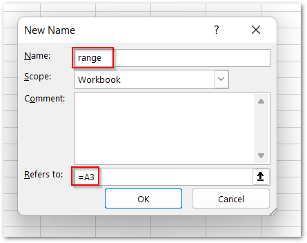
Here we have removed the $ sign that made the absolute referencing. A3 is two rows below cell A1. If we refer to the “range” in any cell i.e C1 then it would refer to cell C3.

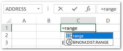
Hit enter key.

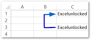
The formula in cell C1 is =range which becomes equivalent to =C3.

Consequently, this brings us to the end of the blog.

Thank you for reading.