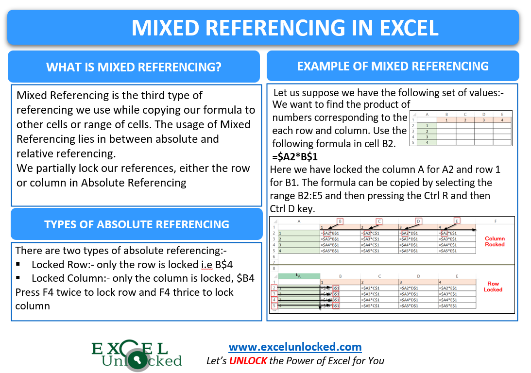
In the earlier blogs, we did the usage of Relative and Absolute Referencing. Mixed Referencing is the third type of referencing we use while copying our formula to other cells or a range of cells. The usage of Mixed Referencing in Excel lies in between the Relative and Absolute Referencing. We highly recommend reading about Relative and Absolute Referencing before going on to Mixed Referencing.
So let us start learning.
What is Mixed Referencing in Excel?
As the name suggests to you, Mixed referencing is a combination of both absolute and relative referencing.
- Absolute Referencing – We lock both the Column and Row forming the cell referencing so that it does not change when we copy the formula.
- Relative Referencing – The cell references, both row, and column can change depending on where you copy your formula.
So the definition of Mixed referencing becomes, that we can freeze either the row or column forming the cell reference and either of them would not be locked.
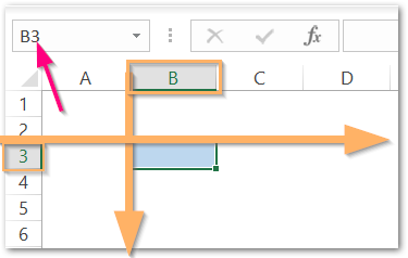
As we know a cell is made by the intersection of one row and one column. For example, the intersection of Column B and the 3rd row forms the cell B3
Types of Mixed Referencing
There are two subtypes of Mixed Referencing in Excel as follows:-
- Locked Row – In this, we lock the row number of our cell reference. For example, when we copy the formula containing B$3 ( only row number is locked ), to the right it becomes C$3 ( column changed) but when we copy it down, it remains B$3 (row didn’t change and becomes B4)
- Locked Column – In this type of reference. we lock the column name for our cell reference. For instance, when we copy the formula containing $B3 ( only column B is locked), to the right (it remains $B3 ( column didn’t change and become C3 ) but when we copy it down, it changed to $B4 ( row changed as only the column was locked )

How to Apply Mixed Referencing
The following are the steps to apply mixed referencing to our formulas in excel:-
- Press = sign and start typing any function name. For instance =AVERAGE(
- Once you start the parenthesis, select the function arguments i.e B3
- Press F4 twice to lock the row and B3 would become B$3
- Now type : and then select cell D6. To lock the column of cell D6, press the F4 key thrice. It will update to =AVERAGE(B$3:$D4)
Now when you will copy the formula to any range, both the mixed references will work correctly.
Example of Mixed Referencing
Let us suppose we have the following set of data as mentioned below:-
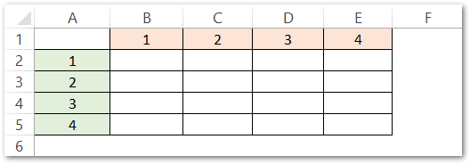
Now we want to find the product value in the range B2:E5 that corresponds to the row and column. Type in the following formula in cell B2:-
=$A2*B$1
Or you can:-
- type = and left arrow key to go to cell A2. Press the F4 key thrice to lock the column for A2.
- Add the * sign and then press the up arrow key to select cell B1. Press the F4 key twice to lock the row for B1. hit enter
After this, you need to copy this formula to the entire range:-
- Select the range B2:E5. Press the Ctrl R key and then the Ctrl D key to get the formula results.
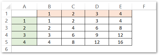
You can press the Ctrl ~ ( tilde ) to see the formulas behind the formula results in your spreadsheet to see what happened when we copied the formula.
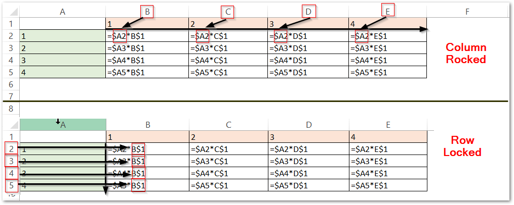
So this image clearly explains that the Column for cell A2 has been locked while the Row for cell B1 is locked when copied to right and down respectively.
This brings us to the end of the blog. Thank you for reading.

