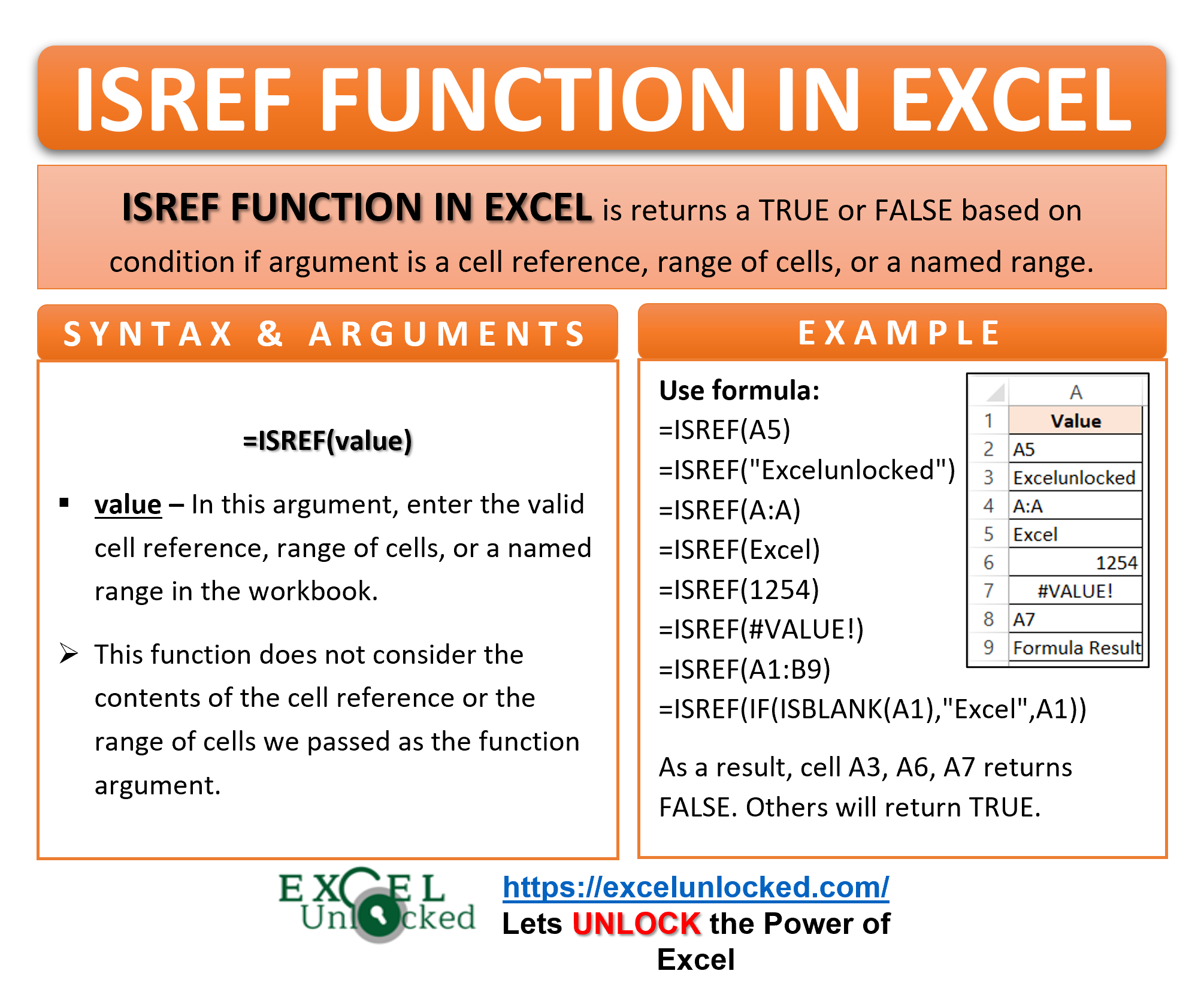
A cell reference refers to the specific address of each cell in the spreadsheet. The column number is represented by alphabets from A to XFD while there is a serial number for each row in Excel. In the cell address, first comes the Column alphabet, and thereafter is the row number i.e A1 (cell where the column A and row 1 intersect). The ISREF Function of Excel is all about references.
These cell references can be the result of many other formulas like the OFFSET Function, INDEX Function, or INDIRECT Function. This is when the use of the ISREF comes.
Here we go 😎
When to Use Excel ISREF Formula
The word ISREF represents “Is it a cell reference?”. The ISREF function returns a logical TRUE or FALSE based on the condition if the passed argument is a cell reference, range of cells, or a named range.
This function can check if the result of any other formula is a cell reference or not. This function is categorized under the Information Functions of Excel.
Syntax and Arguments
=ISREF(value)
The below point explains the required function argument for Excel ISREF Formula.
- value – This is the argument for which we want to check for a valid cell reference, range of cells, or a named range in the workbook.
There is no optional argument in the ISREF Formula.
Points to Remember About ISREF Function
The following points should be kept in mind while using the ISREF formula.
- This function does not consider the contents of the cell reference or the range of cells we passed as the function argument.
- In Excel, The last column of the spreadsheet is XFD and the last row is 1048576. After that, the columns like ZZZ or row numbers like 1532754 will make the cell reference invalid i.e ZZZ5. The function returns a logical FALSE for these typed of invalid cell references.
- We can check if any formula returns a cell reference or not. Just put that formula as ISREF Function argument. A logical TRUE will indicate that the formula successfully found the cell reference we were looking for.
- The ISREF Function will not give any error message, whatever be the function argument. For instance, look at this formula =ISREF(#VALUE!), this will return a logical FALSE.
Examples to Learn Excel ISREF Formula
In this section of the blog, we will perform some practical examples to know more about the ISREF Function of Excel.
Ex. 1 – Simplest Example for ISREF Function of Excel
Let us pass different types of function arguments to get the results for the ISREF formula. Below are the values.
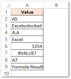
Use the following formulas in order to get the results.
| Formula |
| =ISREF(A5) |
| =ISREF(“Excelunlocked”) |
| =ISREF(A:A) |
| =ISREF(Excel) |
| =ISREF(1254) |
| =ISREF(#VALUE!) |
| =ISREF(A1:B9) |
| =ISREF(IF(ISBLANK(A1),”Excel”,A1)) |
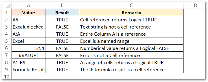
As a result, the formula has returned logical TRUE/FALSE for different function arguments.
Explanation – There is cell reference, an entire column reference, Named range, range in the formula contained in cells B2, B4, B5, B8. Consequently, as a result, the formula has returned a logical TRUE for them.
The cells B3, B6, B7 contain a text string, numerical value, and an error. Therefore the formula returns a Logical FALSE for them.
Cell B9 contains an IF formula, the condition for the formula is TRUE and therefore the formula returns a cell reference. As the IF formula result is a cell reference when it is passed as the ISREF Function argument, It returns a logical TRUE.

Ex. 2 – Using INDIRECT Formula with ISREF to Check the Validity of a Named Range
The INDIRECT Function of Excel converts the text strings into cell references. As a result, the INDIRECT Function generates a cell reference if it is valid otherwise, it returns a #REF! error.
In this example, let us say we have the sales of two companies named Fashion Look and New Fashion. Below are the order details.
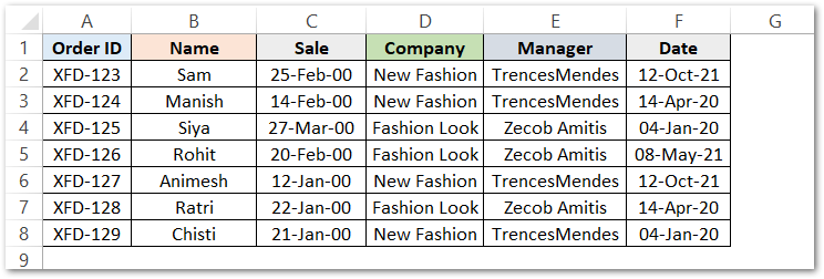
Now, first of all, we will create named ranges for all the columns from A to F.
Below are the steps to create named ranges for all columns at once.
- Select the range of cells A1:F8.
- Press Ctrl+Shift+F3 to open the Create Names From Selection Dialog Box.
- Select Top Row. This will name the ranges using the first row (A1 to F1) as the name of the ranges containing the data of cells under them.
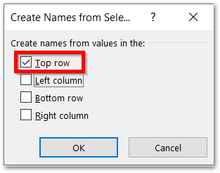
As a result, we can check if the named ranges have been created as valid cell references using this Formula. Use the following formula.
=IF(ISREF(INDIRECT(C12)),"Exists","Not Exists")
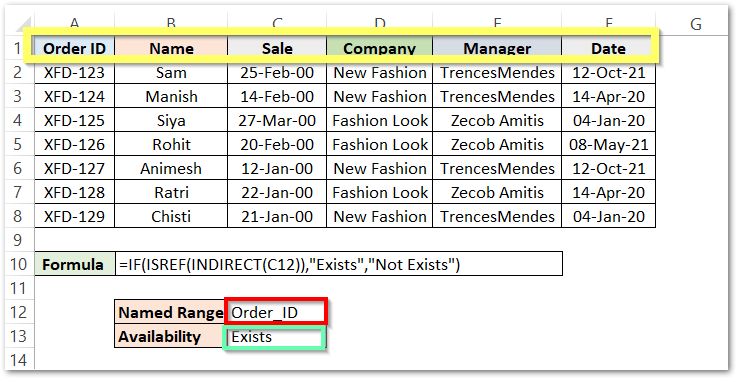
The range of cells in the yellow box contains the name of the range for each of those columns (A to F).
The Red Box contains the named range whose validity we want to check for.
Green Box contains the Status of the named range entered in cell C12.
As a result, the formula has returned a text string “Exists” for the named range Order_ID.
When We enter a named range like Customer ID in cell C12. This happens to be the result.
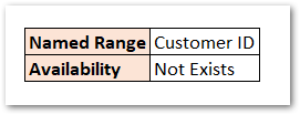
As a result, the formula told us that this named range does not exist i.e we never created this range in this workbook.
Step by Step Explanation
Explanation – Let us see in steps, how does the formula work.
- The IF formula has a condition ISREF(INDIRECT(C12)).
- If this condition returna a logical TRUE, then the formula gives a text string “Exists”.
- If this condition returns a logical FALSE, then the formula gives a text string “Not Exists”.
Now the condition contains an INDIRECT Function having C12 as the input argument. The INDIRECT Function will check if the text contained in cell C12 is a valid reference or not. The function will return a reference to the named range if it is valid, otherwise, it returns an error.
When we entered Order_ID in cell C12, the INDIRECT Function picks the text string from C12 and creates a reference to that range. As a result, the ISREF formula returned a logical TRUE because its input argument is a reference to a named range (A2:A8). The condition is TRUE and the result is a text string “Exists”.
Thereafter when we tried to check the validity for Customer ID as the cell reference, the INDIRECT Function did not find any reference to it. It returned a #REF! error. After that. the #REF! passed as the function argument of ISREF. The ISREF Function gives a logical FALSE for the Error values. Consequently, the condition becomes FALSE and the IF formula gives a text string “Not Exists”.
With this, we had like to end the ISREF Function blog, but there is so much more to learn.
Thank you for reading 😉
RELATED POSTS
- CELL Function in Excel – Get Information About Cell
- ISERR Function in Excel – Checking If The Cell Contains An Error
- ROW Function in Excel – Get Cell Row Number
- ISERROR Function in Excel – Checking for Errors
- Three Ways to Find Formula Cells in Excel
- ADDRESS Function in Excel – Get Excel Cell Address

