Many times, while working with numeric data in excel, we might feel a need to check if the cell contains a number or not. Manually going to each cell and checking if cell contains a numeric value is not a good option to go with. Interestingly, excel has an inbuilt formula to achieve this, viz. ISNUMBER function in excel.
In this tutorial, we would learn how to use the ISNUMBER excel function, using simple examples.
Here we go 😎
When To Use ISNUMBER Function of Excel
The expression ISNUMBER denotes “Is it a number?”.
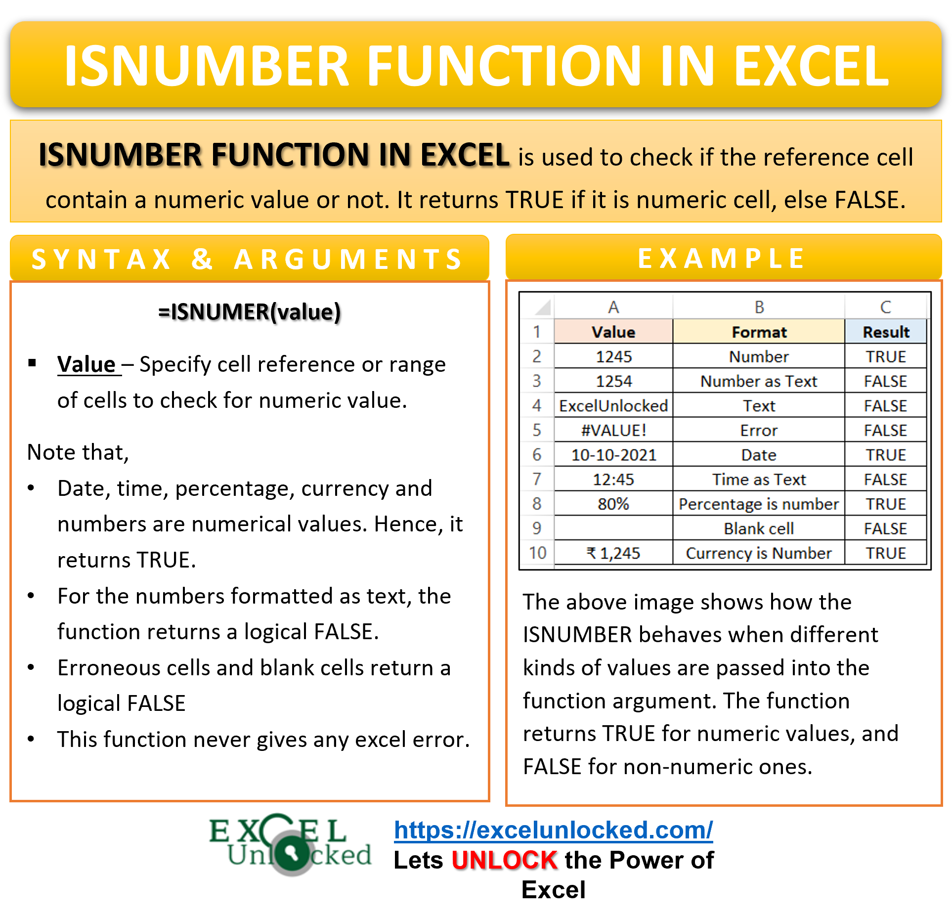
To put it simply, the ISNUMBER formula of excel checks if the passed function arguments contain a numerical value or not. As a result, the function returns a logical TRUE if the cell contains a numerical value, else it returns a FALSE.
The ISNUMBER formula is a part of the Information Functions of Excel.,
Syntax and Arguments
=ISNUMBER(value)
The below point explain the required function argument for ISNUMBER Function.
- value – In the value argument, specify a cell reference, the range of cells, or a formula result for which you want to check for the numerical value.
Points To Remember About ISNUMBER Function of Excel
The following points must be kept in mind before the actual usage of the ISNUMBER Formula.
- The date, time, percentage, currency and numbers, all are the forms of numerical values. Consequently, the ISNUMBER function will return ‘TRUE’ (see example 1 below).
- For the numbers formatted as text, the function returns a logical FALSE.
- The function is a form of IS Functions. It only analyzes the data and never gives any excel error.
- Erroneous cells and blank cells return a logical FALSE (see example 1 below).
Examples to Learn the Usage of ISNUMBER Formula
Let us perform some practical examples to learn the usage of the ISNUMBER function.
Ex. 1 – Simplest Example for Excel ISNUMBER Formula
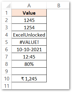
In this example, we will pass different arguments to the ISNUMBER Function to check if the cell contains a numerical value or not. Below are the values.
Use this ISNUMBER formula to get the results.
=ISNUMBER(A2)
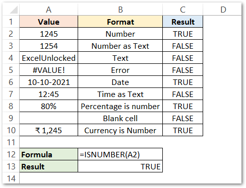
As a result, The ISNUMBER formula returns ‘TRUE’ for cell A2. Now, use the Excel fill handle tool to copy the formula down the column.
Explantation – For the cells A2 and A3, although they both appear to be numbered, the ISNUMBER function argument returns different results. This is so because the value in cell A3 is not a number formatted value, but a text format. So by using the formula, we can differentiate between numbers and numbers formatted as text.
Similarly, A6 and A7 results are different. This is so because A6 contains a date that will is considered as a number. Whereas, cell A7 contains time formatted as text, which will FALSE, as it is a non-numerical value.
Text string in Cell A4 returns a logical FALSE because it is not a numerical value whereas cell A5 also returns a logical FALSE because an error cannot be considered as a numerical value.
A blank cell A9 contains no numerical value, thus it also returns a Logical FALSE.
Cell A8 and A9 are the numbers in percentage and currency format which makes the function return a Logical TRUE.
Ex. 2 – Applying Data Validation To Enter Numerical Entries Only
Data validation refers to limiting the types of values we can enter in a cell. In simple words, it is the validation of data in the excel cell.
For example, we might want the user to enter the marks of students in numerical format only. No other format is permitted.
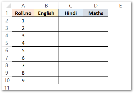
We will do data validation on the marks columns. Follow these steps.
- Select the range of cells (B2:D10).
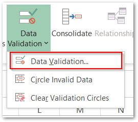
- Go to Data Tab> Data tools Group> Data Validation.
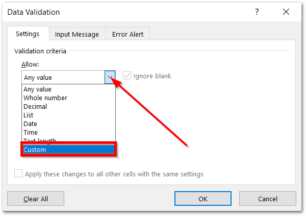
- The Data Validation dialog box appears. From the Allow drop down menu, choose Custom, as shown below.
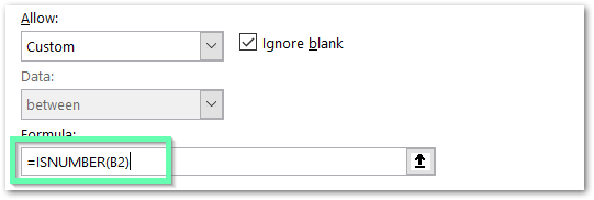
- Enter this formula in the empty formula block.
=ISNUMBER(B2)
- Click on Ok.
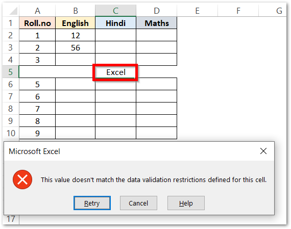
Now when you try to enter any value in the range B2:D10 other than a numeric value (for example, a text string), excel will consider it as an invalid cell entry. As a result, it will return the following error popup box.
Ex. 3 – Using FIND and IF Formula With ISNUMBER Function Of Excel
Let us say we have a clothing store. Each type of cloth is named in a format like this: item-size-color. Below is the variety of clothing available at the store.
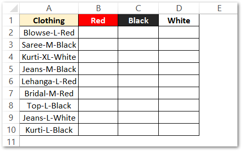
The owner of the shop wants to know the availability of variety for each of red, black and white color. We will use these formulas containing the FIND and IF function of Excel in columns B, C, D for Red, Black, and White clothing.
=IF(ISNUMBER(FIND($B$1,A2)),"x"," ")
=IF(ISNUMBER(FIND($C$1,A2)),"x"," ")
=IF(ISNUMBER(FIND($D$1,A2)),"x"," ")
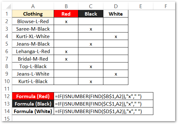
As a result, the formula has returned “x” for the different colored clothing available in the store.
The $ locks the cell reference when we copy the formula for the rest of the records. This is known as absolute cell referencing.
Explanation – Let us see in steps how did the formula work.
- The IF formula has a condition ISNUMBER(FIND($B$1,A2)). If this condition is TRUE then the Formula returns “x” or else ” ” (blank cell).
- The IF condition has two functions used:-
- In the FIND Function, find_text is $B$1 ( locked for the column C ) that contains a text string “Red”. The within_text is cell A2 (moves one cell below each time we copy the formula). The FIND Function returns the numerical position of the substring Find_text argument in the main string Within_Text if it exists otherwise it returns a #VALUE! error.
- When the FIND Function finds the position, a numerical value returned makes the result of ISNUMBER formula TRUE ( condition becomes TRUE ). When the FIND function does not find the substring in the main string, it returns a #VALUE! error, which when passed to the ISNUMBER Function, makes the IF condition FALSE.
Usage of Absolute Referencing
For cell B2, the result is “x”. The condition is TRUE as cell A2 (main_string) contains the substring in cell B2. The FIND Function returns 10 as the position of “Red” in “Blouse-L-Red”. When 10 is passed as the function argument of the ISNUMBER formula, the condition is TRUE and the entire formula returns “x”.
Once we copy the formula to cell B3 it becomes:-
=IF(ISNUMBER(FIND($B$1,A3)),"x"," ")
The Cell Reference ( substring ) remains the same because of absolute referencing in $B$1 whereas the cell A2 changes to A3. The Clothing shifts one cell down because it has no absolute (fixed) referencing.
We used the same concept for black and white clothing types. The Absolute referencing shifts to $C$1 and $D$1 for the column C and D. This is to change the substring we want to look for i.e black in column C and white in column D.
Thank you for reading 😉

