ISTEXT Function in Excel – Checking if Cell Contains Text

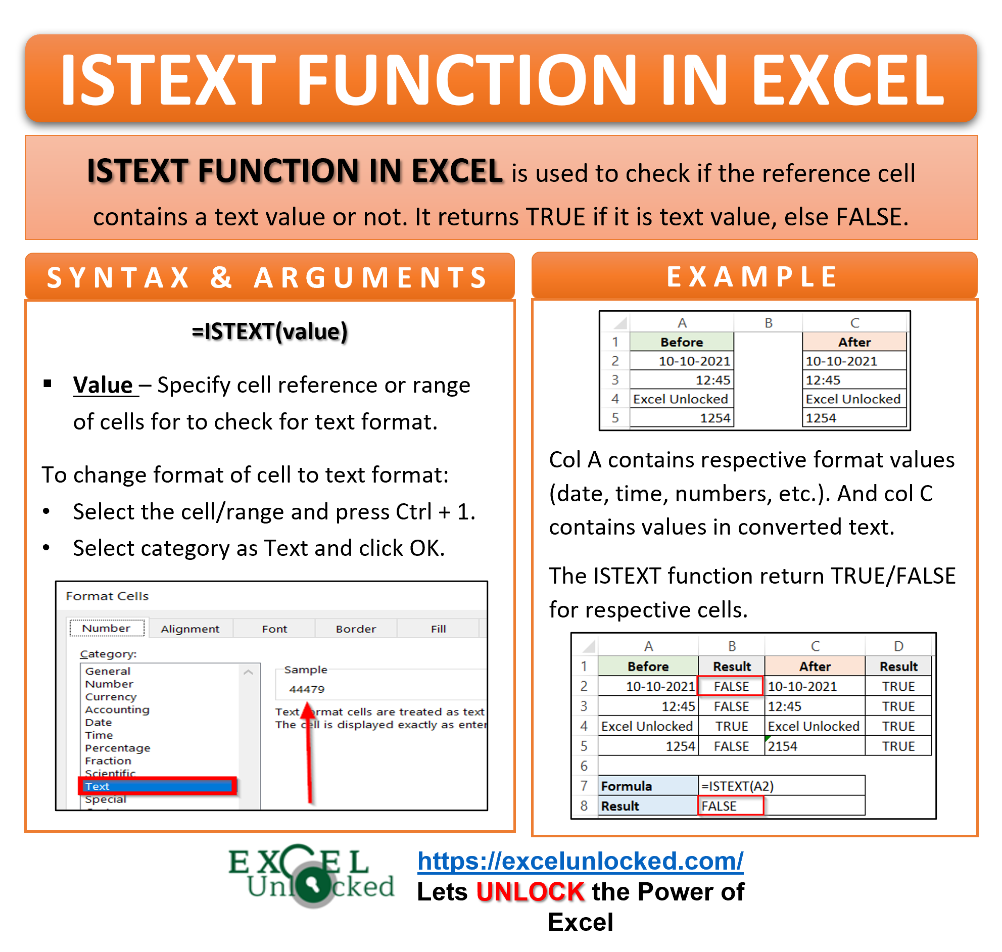
Whenever we are working with data in Excel, we have to work with the cells set to text format. The text strings, numbers, date, time, or any value can be set to text format. In this tutorial, we would learn about how to use the ISTEXT Function in Excel to check if a particular cell contains a text or not.

Here we go 😎

When to Use ISTEXT Formula in Excel

The expression ISTEXT represents “Is it text?”. The ISTEXT excel formula helps us to check if the cell is set to a text format or not.

The function returns a ‘TRUE’ if the passed argument is in text format, otherwise, it returns a ‘FALSE’.

The ISTEXT Function is a part of the Information functions of Excel.

Usage of ISTEXT Function in Excel

The function when used with the SUM function of excel can count the total number of cells containing text.

We can also use this function before using the TEXTVALUE or DATEVALUE function to check for the text format. Check the TIMEVALUE Function blog (example 2) for that.

Many excel users use the ISTEXT function along with the data validation.

Syntax and Arguments

=ISTEXT(value)

The below point explain the required function argument for the ISTEXT Function of Excel.

• value – In this argument represent the cell reference or the range of cells for which we want to check for text format.

Before going deep into how the excel ISTEXT formula works, let us see how to convert a cell format to text.

How to Change Cell Format To Text Format

In this section, we will learn to change the cell format to text. Let us say we have a date, time, text strings, and number in a range of cells in their respective formats. Follow the below steps:

• Select the range (A1:A4) and hit Ctrl + 1 to open the format cells dialog box.
• Select the category as ‘Text’ and thats it.

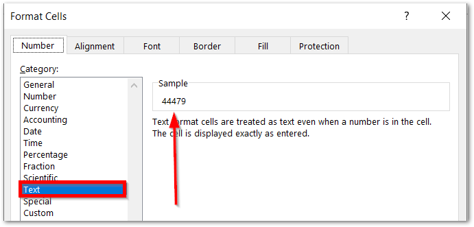
• Click on OK.

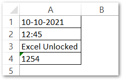
As a result, the values get converted to text format.

The time and date convert into the text format. As you can see all the values are left aligned, which denotes that they are in text format.

Examples to Learn Usage of ISTEXT function of Excel

In this section of the blog, we will be performing some practical examples to learn using the ISTEXT function in Excel.

Ex. 1 – Simplest Example to Learn ISTEXT Formula of Excel

The below image shows how the cell content looks like before and after changing the cell format to text. Below are two ranges of cells.

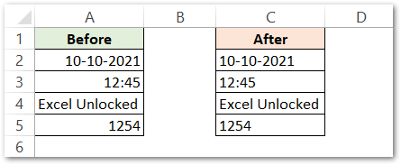
The first range A2:A5 represents the cells in their respective cell formats whereas the range C2:C5 is formatted to text format.

Use this formula to check the results.

=ISTEXT(A2)

Use this for formatted range (D2)

=ISTEXT(C2)

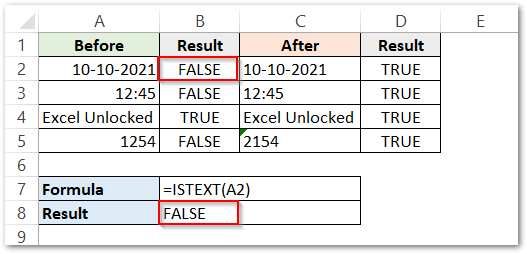
As a result, the formula returns ‘FALSE’ for range A2.

Use the autofill handle tool to copy for the remaining cells.

Explanation – The cell format of Cell A2, A3, and A5 are date, time, and number. On these cell value, the ISTEXT function returns ‘FALSE’. On the other hand, cell A4 contains a text string “Excel unlocked”, so the formula returns ‘TRUE’.

All the values in column C are in text format. Although the date, time number appears as non-text values, the ISTEXT function return ‘TRUE’ for all cells of range C2:C5.

The green arrow at the top left corner of cell C5 indicates the number formatted as text.

Ex. 2 – Counting Total Number of Cells Containing Text

In this example, let us say we have the marks of students of a class. There are few who are either absent or on a leave.

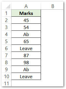
Let us say we want to find the number of students who did not attempt the exam (i.e. absent or on leave).

Use this formula to get the results.

=SUM(--ISTEXT(A2:A10))

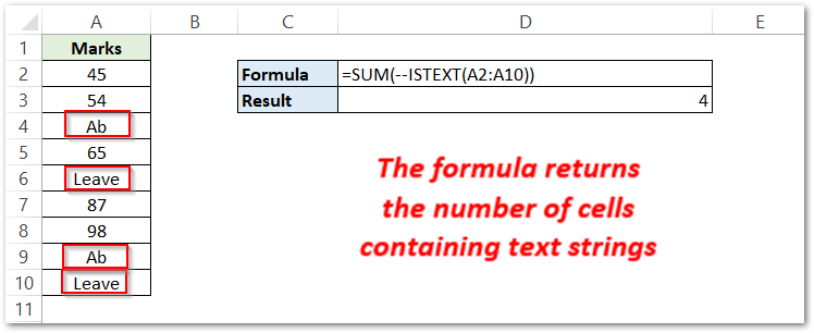
As a result, the formula returns 4.

Explanation – Let us break this formula into parts to see how we reached the result.

• We have passed a cell range to the ISTEXT formula. The part ISTEXT(A2:A10) checked each of the cell in the range and returned an array containing TRUE/FALSE like this {FALSE;FALSE;TRUE;FALSE;TRUE;FALSE;FALSE;TRUE;TRUE}.

• The Unary Operator (–) used before the ISTEXT Formula changes TRUE and FALSE into 1 and 0. So the array returned by ISTEXT Function becomes {0;0;1;0;1;0;0;1;1}

• After that, the SUM function finds the sum of elements of the arrays. 0+0+1+0+1+0+0+1+1=4.

Ex. 3 – Applying Data Validation Rule For Text Values Only

Data validation is a useful feature in excel to configure validation of values in excel. When data validation is applied to a cell, the users can only fill certain values. In data validation, you need to specify a condition. If the entered value in the cell the condition TRUE, only then the value is validated otherwise the user will see an error message.

In this example, let us say we have the order details of a company and we want the user to fill into it the order amounts in words only. For example – Two Thousand and Five Hundred Rupees

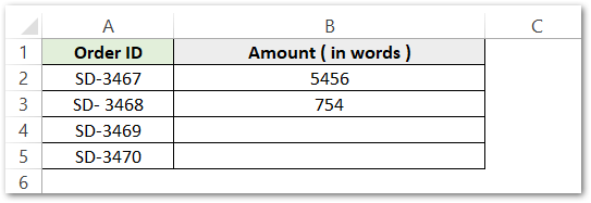
Until now, we can enter the amount in numbers (cell B2 and B3 ).

Follow these steps to restrict the data values to be entered in the amounts column.

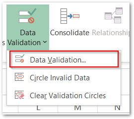
• Select the range of cells (B2:B5) on which you want to apply validation. Go to Data Tab> Data tools Group > Data Validation Button. Choose Data Validation from the drop down menu.

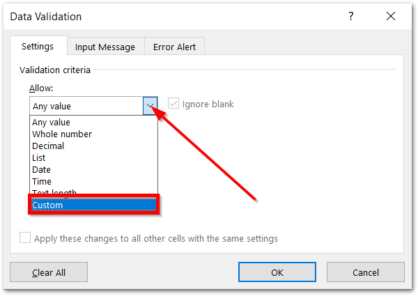
• The Data Validation Dialog box appears. After that, choose custom from the drop-down menu.

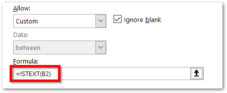
• Enter this formula in the ‘Formula’ box. From now, only those values will be valid in cell B2 that makes this formula return ‘TRUE’.

=ISTEXT(B2)

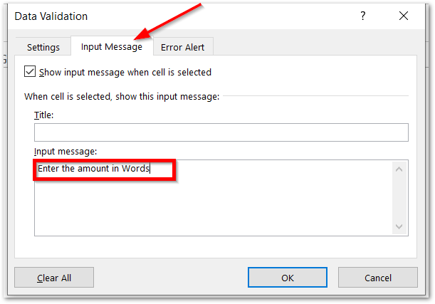
• Go to ‘Input Message’ tab and enter the message to display.

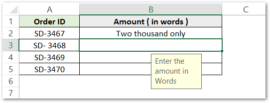
• Now the user will also see this message to remind him about the validation of data.

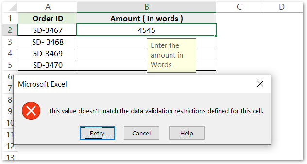
• And in case, if the user enters any value that is non-text, there will be this error message popping up on the screen not accepting that value.

This brings us to the end of the ISTEXT Function blog.

Thank you for reading 😉