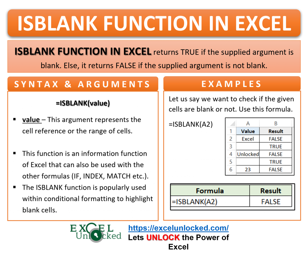
Many times, while analyzing the data in excel, we might be willing to work with the blank cells in the data. Out of the whole big data in excel, we may feel a need of finding only the blank cells using a formula. This is when the ISBLANK function of Excel comes into its use.
In this article, we would go through the ISBLANK formula in excel and cover all the aspects of this information function. This tutorial includes the purpose of excel ISBLANK formula, function syntax and argument, and examples.
Here we go 😎
When To Use ISBLANK Function in Excel
The expression ISBLANK denotes “Is the cell blank?”. ISBLANK formula of excel returns a TRUE or FALSE if the entered argument is a blank cell or a non-blank cell respectively. The function is categorized under the information functions group of Excel.
Whenever we want to highlight the blank cells in a range, ISBLANK Function comes into its use. We can use the function to perform conditional formatting as well as with other excel functions.
Syntax and Arguments
=ISBLANK(value)
The below point explain the required function argument for the ISBLANK function of Excel.
- value – In this argument, specify the cell reference or the range of cells for which you want to check the blank cell.
The ISBLALNK Function can be used in nesting of functions with IF formula (example 3 in this blog) as well as with the INDEX/MATCH combination (example 4) or even with the HLOOKUP Formula.
Examples To Learn ISBLANK Formula of Excel
In this section, let us learn the usage of the excel ISBLANK function using some classic examples. This section explains how the ISBLANK excel formula works in excel.
Ex. 1 – Simplest Example to Learn Excel ISBLANK Formula
In this example, we will check the result of the ISBLANK Function for some empty and non-empty cells.
Below is the sample data.
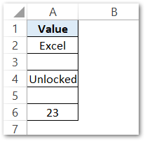
To check if the cell is blank or not, simply type the following formula for cell A2, and drag it to other cells below.
=ISBLANK(A2)
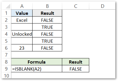
As a result, the formula returns a boolean value ‘FALSE’.
Explanation – The cells A2 and A4 contain text string (i.e. non-blank cells). Therefore, the formula returns ‘FALSE’. Cell A6 contains a number 23 (a non-blank cell), therefore ISBLANK Function returns ‘FALSE’. The cells A3 and A5 return a TRUE because they are empty cells.
Ex. 2 – Using Conditional Formatting with ISBLANK Function
This example will help you to understand how to use the ISBLANK function to highlight the blank cells in excel.
Let us say we have a list containing the marks of classroom students. For the students who were absent on the day of the exam, the marks block is empty.
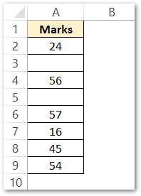
Follow these steps to do conditional formatting on this range of cells, and highlight blank cells in excel.
- Select the range of cells (A2:A9) and navigate to the ‘Home’ tab > ‘Style’ group > ‘Conditional formatting’ Button, as shown below:
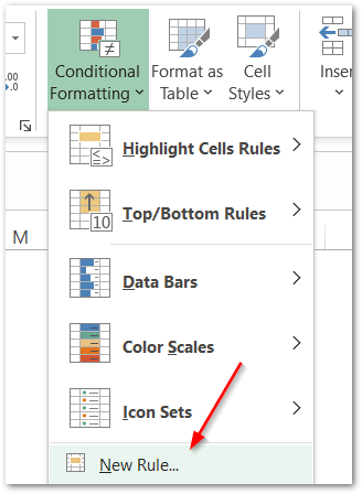
- Click on ‘New Rule’ option. Click on “use a formula to determine which cells to format” button and enter this formula in the provided space.
=ISBLANK(A2)
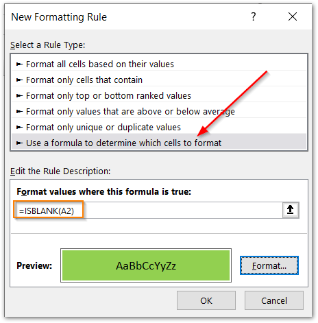
- Choose the desired format for the cells that return ‘TRUE’ (Blank cells). In this example we have set the format to solid green color fill.
- Finally, click on OK and here are the results.
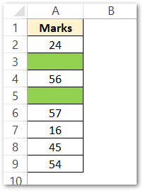
Explanation – The formula has successfully highlighted the blank cells. In this case, the formula is =ISBLANK(A2) and the cell formula is solid green. Therefore, when the formula returns TRUE for a non-blank cell, the cell format is changed to a solid green.
This is how we can use a formula to solve the problem on how to highlight blank cells in excel 😉
Ex. 3 – Filling Cells Based on Result of ISBLANK Function of Excel
Let us now move one step ahead. In this example, we will learn to mark the attendance of the students using excel formula.
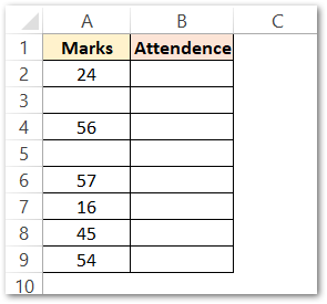
Enter the following formula in cell B2.
=IF(ISBLANK(A2),"ab","p")
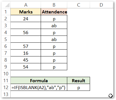
As a result, the formula returns “p”.
Drag the formula down to other cells in column B and see the results.
Explanation – The above formula is very easy to understand if you know how does IF function0 works in Excel. In this formula, the condition to check in the IF formula is the formula: ‘ISBLANK(A2)’. If cell A2 is blank, It will return a boolean TRUE or else FALSE. IF the result of the ISBLANK function is TRUE, then the formula will return “ab”. Else, if the result of ISBLANK is FALSE, the IF function returns a “p”.
In this example, A2 is a non-empty cell, the ISBLANK Formula returns a FALSE. The result of the IF formula becomes “p”.
Ex. 4 – Using ISBLANK Function to Extract First Non-Empty Cell Value
Let us say we have the following data in excel and we would like to extract the value of the first cell that is filled.

To achieve this, we need to use the nesting of the formulas MATCH and ISBLANK.
We will start by using the MATCH Function of Excel. Use this formula to get the position of the first non-empty cell in the range A2:D2.
=MATCH(FALSE,ISBLANK(A2:D2),0)
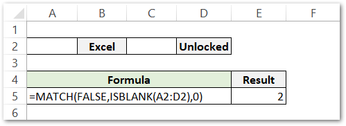
As a result, the formula returns 2.
Explanation – In the above MATCH Formula, we have passed the lookup value to be FALSE. The lookuo_array is the result of the array of elements returned from the formula ISBLANK(A2:D2). The formula array of elements TRUE, FALSE, TRUE, FALSE. We have set the function to exact match (0) for the matching of lookup_value in lookup_array. The FALSE encounters at the second position in the lookup_array (TRUE, FALSE, TRUE, FALSE ). So the result of the formula becomes 2.
Once you have entered the above formula, press ctrl+shift+enter to get the result (2) for the array function. In case if you hit Enter after typing the formula, It will return a #N/A error.
Now, After finding the position of the first non-empty element, we will extract the actual value at that position. Use the following INDEX formula of Excel merged with the above MATCH formula.
=INDEX(A2:D2,MATCH(FALSE,ISBLANK(A2:D2),0))
The result will be the same if we put the output of MATCH Formula in the INDEX formula
=INDEX(A2:D2,2)

As a result, the formula has returned a text string “Excel”.
Explanation – In the INDEX formula, we have passed the array A2:D2. The result of the MATCH formula will act as the row_num of the INDEX function. The formula has returned the first non-empty element from the array of Cells.
Bonus Section for ISBLANK Function
In excel, there can be the cells returning a blank string. We can use the following formula to get an empty string.
=""
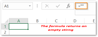
Use the following formula, to see if the ISBLANK Formula considers it to be an empty cell or not.
=ISBLANK(A1)
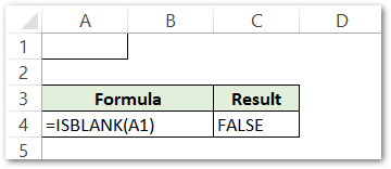
As a result, the formula returns a FALSE.
Explanation – We have passed the value as cell A1 to the ISBLANK Formula. Cell A1 looks to be empty but it is not. We have entered an empty string in cell A1 which makes it non-empty, thus the formula returns a boolean FALSE.
And with this, our blog comes to an end.
Thank you for reading 😉
RELATED POSTS
- ISNONTEXT Function of Excel – Check Non Text Cell in Excel
- ISNUMBER Function of Excel – Checking If Cell Contains a Number
- Empty Cells VBA – Check, Count, and Highlight
- How to Enter Text in Blank Cells in Excel
- Three Ways to Find Formula Cells in Excel
- ISTEXT Function in Excel – Checking if Cell Contains Text

