The MATCH function in excel is very commonly used formula in excel to find the position of a particular cell in excel range or array.
In this blog, we would unlock how the MATCH excel function works. We would also cover the formula syntax and argument along with some examples for understanding.
Here we go 😎
When to Use MATCH Excel Function
The MATCH formula is a very useful excel function to find or get the position of the value or text in a particular range or array.
This formula returns a whole number like 1, 2, 3, and so on, wherein these whole number denotes the cell position of the lookup value.
Syntax and Arguments
=MATCH(lookup_value, lookup_array, [match_type])
This formula has three arguments:
- lookup_value – In this argument, specify the value or text that you want to search for in a particular rage of cells.
- lookup_array – In this argument, specify the cells range or array in which you want to search for lookup_value.
- [match_type] – It is an optional argument wherein you specify how excel should perform the matching activity. It can take -1, 0, or 1.
Use of [match_type] Argument in MATCH Excel Formula
The [match_type] argument of the excel function is an optional argument wherein you specify how the excel should perform the matching activity.
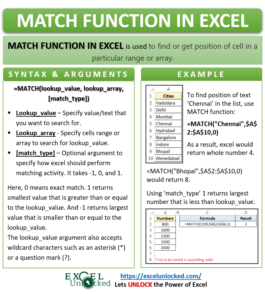
- 0 – If you specify [match_type] as 0, then excel would search for the exact match of the lookup_value in the lookup_array.
- 1 – The [match_type] 1 returns the largest value that is less than or equal to the lookup_value. For this, the lookup_array must be sorted in ascending order. If you do not specify the [match_type] argument, then excel by default considers it as 1.
- -1 – The [match_type] -1 returns the smallest value that is greater than or equal to the lookup_value. For this, the lookup_array must be sorted in descending order.
Examples of MATCH Formula in Excel
1# Using MATCH Function in Excel with Exact Match
The image below consists of list of Indian cities.
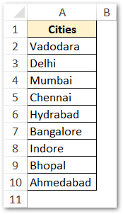
Use the below formula for finding the position of a particular value (for example Chennai) in the range of cells.
=MATCH(“Chennai”,$A$2:$A$10,0)
As a result, excel would return the whole number 4. This is so because the text ‘Chennai’ is in the fourth position in the cell range.
Similarly, =MATCH(“Bhopal”,$A$2:$A$10,0) would return 8.
Instead of using the lookup_value as text, you can even use cell reference, as demonstrated below:
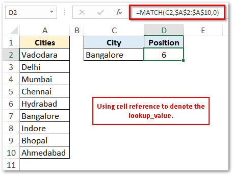
2# Using MATCH Function in Excel with Approximate Match
Now, when you have clearly understood how the excel MATCH formula works with an exact match of lookup_value in the lookup_table, let us see an example on approximate [match_type] -1 and 1.
These two matching types are generally useful in case of number lookup.
Match Type ‘1’
The match_type as 1 returns the largest number that is less than the lookup_value. Make sure to sort the number list in ascending order.
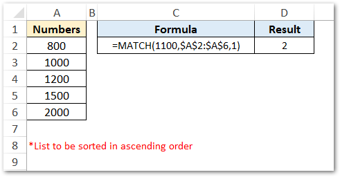
Explanation – In the above example, the match_type is 1. Therefore, the MATCH function returns the position of the largest value below 1100 from the cell range.
Match Type ‘-1’
The match_type as -1 returns the smallest number that is greater than the lookup_value. In this case, make sure that you sort the number list in descending order.
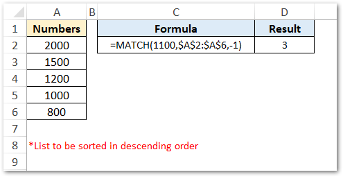
Explanation – In the above example, the match_type is -1. Therefore, the MATCH function returns the position of the smallest value above 1100 from the cell range.
Do Not Miss These Points
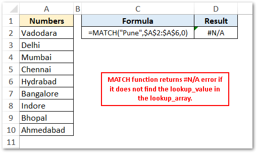
- The MATCH formula in excel gives an excel error code #N/A if it does not find the lookup value.
- Generally, the MATCH function on its own does not give any meaning output. However, this function is very useful when it is combined with other excel functions like the INDEX formula in excel.
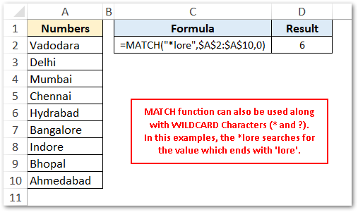
- The lookup_value argument of the MATCH formula also accepts wildcard characters such as an asterisk (*) or a question mark (?).
You can increase your learning by going through the powerful application of INDEX and MATCH Function of Excel – LOOKUP using the INDEX and MATCH formula.
Thank You 🙂
