VLOOKUP and HLOOKUP in Excel

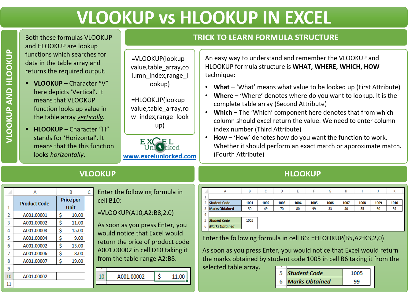
The VLOOKUP and HLOOKUP formula in Excel is the two most important and widely used functions of Excel. These two functions are the lookup functions in Excel that searches for the data in the table array and returns the required output. In this blog, we would learn about these two lookup functions VLOOKUP and HLOOKUP in detail.

Purpose of VLOOKUP and HLOOKUP

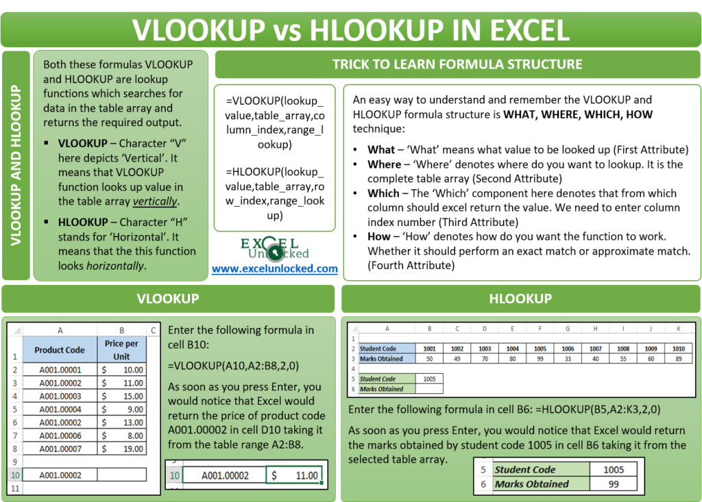
As specified in the introduction paragraph, both these are the lookup functions that search for the data in the table array and returns the output based on this search. The question here arises, that if the purpose of both these formulas is the same, then why has excel provided two different formulas.

A very easy way to know what each of these two functions does is by looking at its first character (V and H).

VLOOKUP – The first character “V” here depicts ‘Vertical’. It means that the VLOOKUP function would look up the value in the table array vertically.

HLOOKUP – The first character “H”, you can guess now, stands for ‘Horizontal’. It means that the this function looks horizontally.

Understanding the Lookup Functionality With Example

Let us take one small example to understand this function in a lay. In the below screenshot you can that in one of the worksheets we have the product code in column A. Column B contains the corresponding price per unit.

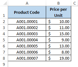
Suppose, in the same worksheet, or some other worksheet, or in some other workbook, you have a product code mentioned. Now, you want to get the price of the product from this table against the product code like this:

The lookup functions would help you to achieve this easily and quickly. Just change the product code and the price would automatically get changed based on the original table array.

Now, when you are aware of the basic difference between the VLOOKUP and HLOOKUP functions and what these would help you to achieve, we are good to start learning each of these formulas and its structure in detail.

VLOOKUP and HLOOKUP Formula Structure in Excel

Both these formula shares a common structure with similar attributes/elements.

=VLOOKUP(lookup_value,table_array,column_index,range_lookup)

Likewise, =HLOOKUP(lookup_value,table_array,row_index,range_lookup)

ExcelUnlocked Trick to Learn Formula Structure

An easy way to understand and remember the VLOOKUP and HLOOKUP formula structure is What, Where, Which, How technique

=VLOOKUP/HLOOKUP(What, Where, Which, How)

1. What – ‘What’ means what value do you want to look up. In our case, it would be cell A2 of the lookup sheet.
2. Where – ‘Where’ denotes where do you want to lookup. It is the complete table array, where the selection of the table should start from the column that contains lookup value. In our case, it is cell range A2:A18 of the sheet that contains the original data table.
3. Which – The ‘Which’ component here denotes that from which column should excel return the value. We need to provide excel with the column index number over here. The counting of the column index number starts from the left-most column of selection array. 
4. How – ‘How’ denotes how do you want the function to work. Whether it should perform an exact match or approximate match. Type ‘0’ or ‘FALSE’ for exact match and ‘1’ or ‘TRUE’ for an approximate match.

Using VLOOKUP in Excel

Among the two, the VLOOKUP is the most used function in Excel. As mentioned earlier in this blog, the VLOOKUP function looks up for the value in the table array vertically and return the corresponding value based on the column index. 

This formula is useful when the records in your data table are arranged in the columnar format.

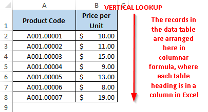
Let us use the ‘What, Where, Which, How’ trick to get the result.

What – In our case, the lookup value is cell A2.

Where – In our case, we want to search for the lookup value in cell range A2:A18 in the original data table. The selection of the range should start from the column which contains lookup value (i.e. column A).

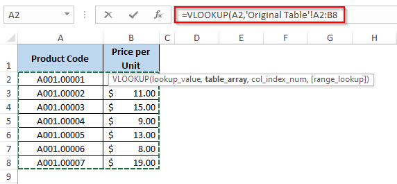
Which – Starting the count from the left-most column (Column A) of the selection, the product price is the comes second. Therefore, we shall type 2 over here.

How – As we want that excel should check for an exact match, therefore, the fourth attribute would be ‘0’ (Or you can even enter FALSE).

As soon as you press the ‘Enter’ key on your keyboard, you would notice that Excel returns the product price based on the product code entered in cell A2 of the lookup sheet. Refer to the screenshot below:

Just change the product code to A001.00003 and you would notice that Excel automatically updates the corresponding product price (taking value from the original lookup table array).

Note that we have used the VLOOKUP formula over here as the original table is in columnar format. Now, when you know how to use the VLOOKUP function, it is very easy to understand the HLOOKUP formula.

Using HLOOKUP in Excel

As mentioned in the introduction, the HLOOKUP function lookups in the table horizontally. Taking an example to understand this better.

As you can see from the above image, the data table is oriented horizontally. The table headings are the row headings.

Therefore, in such a case, the VLOOKUP formula would not work. We need to use the HLOOKUP formula which searches for the value horizontally in the table array.

The ‘What, Where, Which, How’ trick works here as well. Refer to the image shown below:

As a result, you would get the result as below:

Now, just change the student code in cell B5 and the marks obtained would automatically update accordingly.

Keep These Mind While Using VLOOKUP and HLOOKUP

Many a time, while using the VLOOKUP or the HLOOKUP formula, you might have come across an excel error or the value that the formula returned may seem to be an incorrect one.

What are the possible reasons? There are two major points that you need to keep in your mind while working with the excel VLOOKUP or HLOOKUP function, otherwise, the formula would return an error or incorrect value.

Firstly, the lookup value (the first attribute ‘What’) must be the left-most column while selecting the table array (the second attribute ‘Where’).

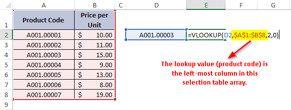
Secondly, there should be unique values in the left-most column in the selection range (just like, in our example, we have a unique product code and unique student code. If there would have been two or more lookup values in the table array, then, in that case, the excel would return the value that comes first in the table array.

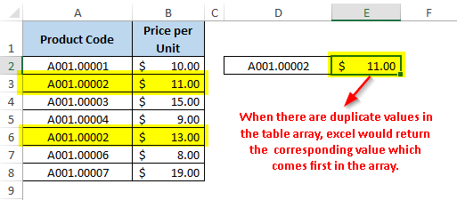
This brings us to the end of this blog. Share your views and comments in the comment section below.