Convert Date To Quarter in Excel

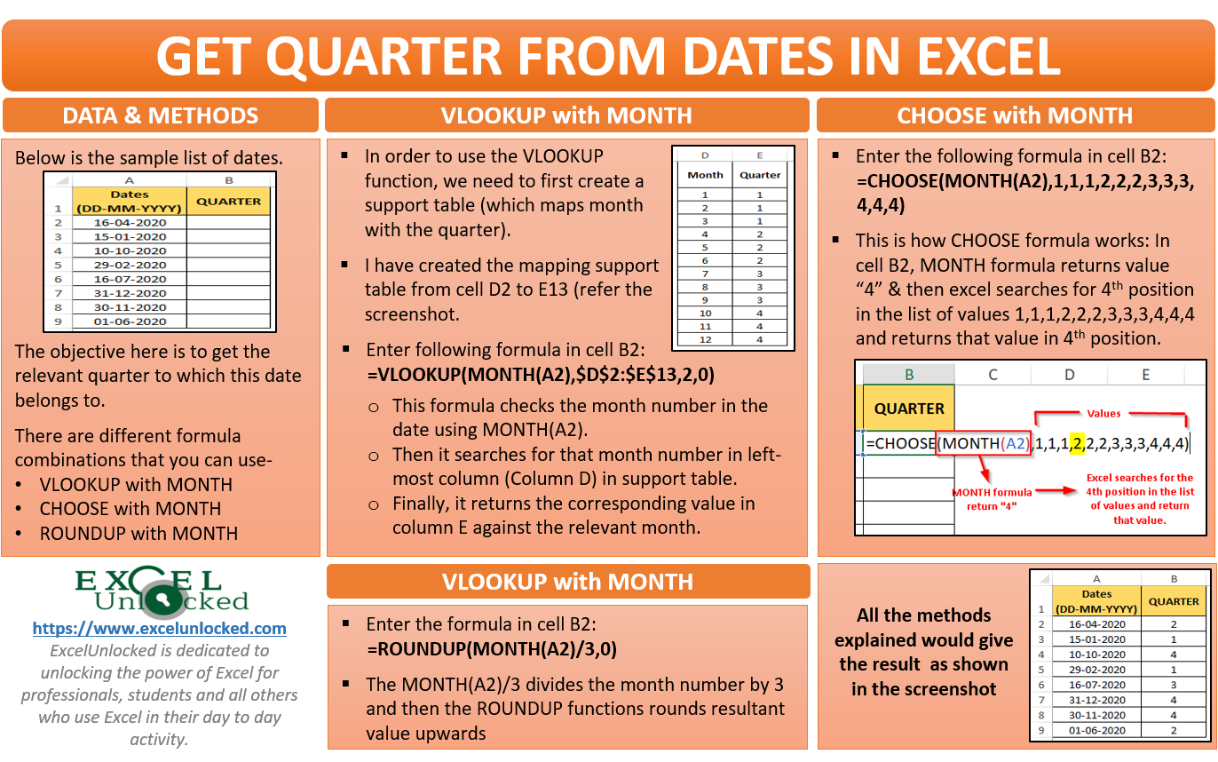
Do you know how to convert a date or a month into the quarter in Excel? In this blog, unlock multiple ways to convert the month into the quarter in Excel. All of the methods that we going to see are formula-based methods. We would be making complex nested formulas to get a quarter from the date.

Sample Dates (Convert Date to Quarter)

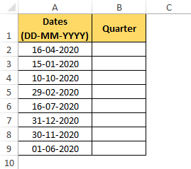
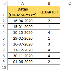
Below is the list of dates that would be used to understand this trick.

Methods to Convert Date to Quarter

As mentioned above, we would be learning different nested formulas to get the quarters from the date. Below is the list-

1. VLOOKUP with MONTH
2. CHOOSE with MONTH
3. ROUNDUP with MONTH

As you can see from all the methods mentioned above, there is one common formula in all (viz. MONTH). 

The MONTH formula returns the month number. It takes only one attribute “cell reference” as its input parameter which means reference of the cell containing the date.

Refer to the below screenshot to understand how is the MONTH formula structured and what does it return as a result.

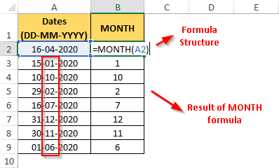
This result will be used in other formulas to get the quarter from this month.

Let us now start learning each of the methods one by one.

VLOOKUP with MONTH Formula

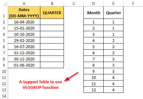
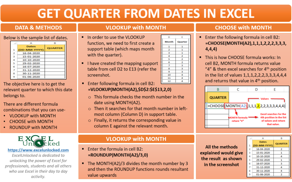
In order to use the VLOOKUP formula, we need to create one table in excel to map the quarter against each of the 12 months.

A support table something like this. It has been made on the assumption that we are using calendar month.

Now, use this formula. Enter it in cell B2:

=VLOOKUP(MONTH(A2),$D$2:$E$13,2,0)

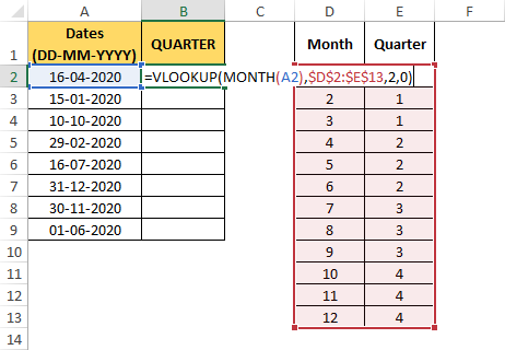
As soon as you press the Enter key, you would notice that the excel returns the quarter number from the date. Excel did a very simple step. Firstly, it checks the month number in the date using MONTH(A2), then it searches for that month number in the left-most column (Column D) in the support table (D2:E13). Finally, it returns the corresponding value in column E against the relevant month.

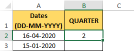
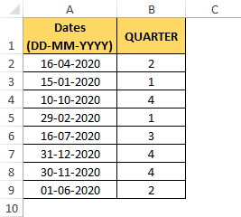
Copy this formula in other cells in Column B to get the result for all of the dates.

CHOOSE with MONTH Formula

Unlike the VLOOKUP formula, we do not need to create any support table for mapping. The formula itself would include the mapping data.

Enter below formula in cell B2.

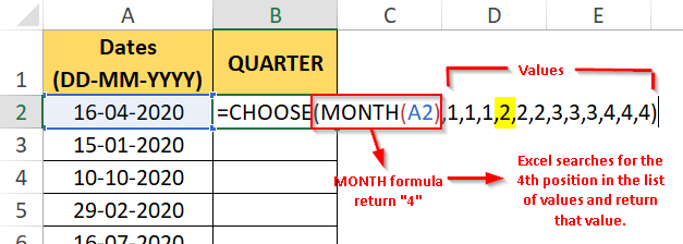
=CHOOSE(MONTH(A2),1,1,1,2,2,2,3,3,3,4,4,4)

The CHOOSE formula reads its first attribute (month number) and returns the value from the series of values starting from the second value based on the position.

As soon as you press Enter key on your keyboard, you would notice that excel returns “2” which is the value mentioned in the fourth position (April) in the CHOOSE formula starting from the second attribute. The below image would explain it in a nutshell.

Now, copy cell B2 and paste it to the other cells in column B. As a result, you would get the quarter for all the dates.

ROUNDUP with MONTH

The ROUNDUP formula is a mathematical formula that rounds the value upwards towards the mentioned number of digits. Enter below formula in cell B2:

=ROUNDUP(MONTH(A2)/3,0)

The first attribute MONTH(A2)/3 divides the month number by 3 and rounds the resultant value upwards.

As soon as you press Enter, the formula would return the quarter from the date.

At last, copy the formula in cell B2 and paste it to the other cells in column B.

But, it is important to note that the above-mentioned methods are just a few that can be used. You can create more using other functions like using the combination of IF and MONTH formula and many more.

This brings us to the end of this blog. I hope that you have learned something out of this blog. Share your views and comments in the comment section below.