How to Hide Formula in Locked Cells in Excel

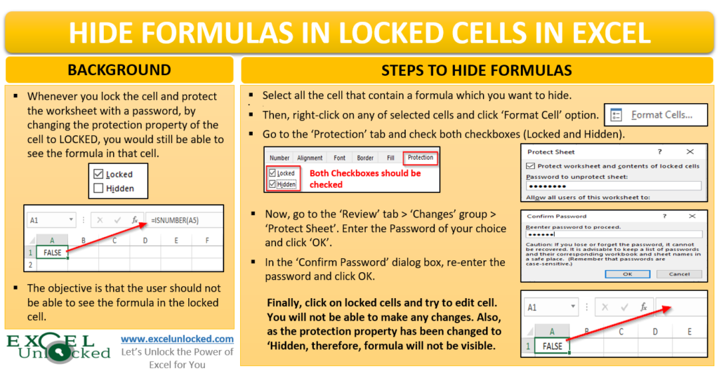
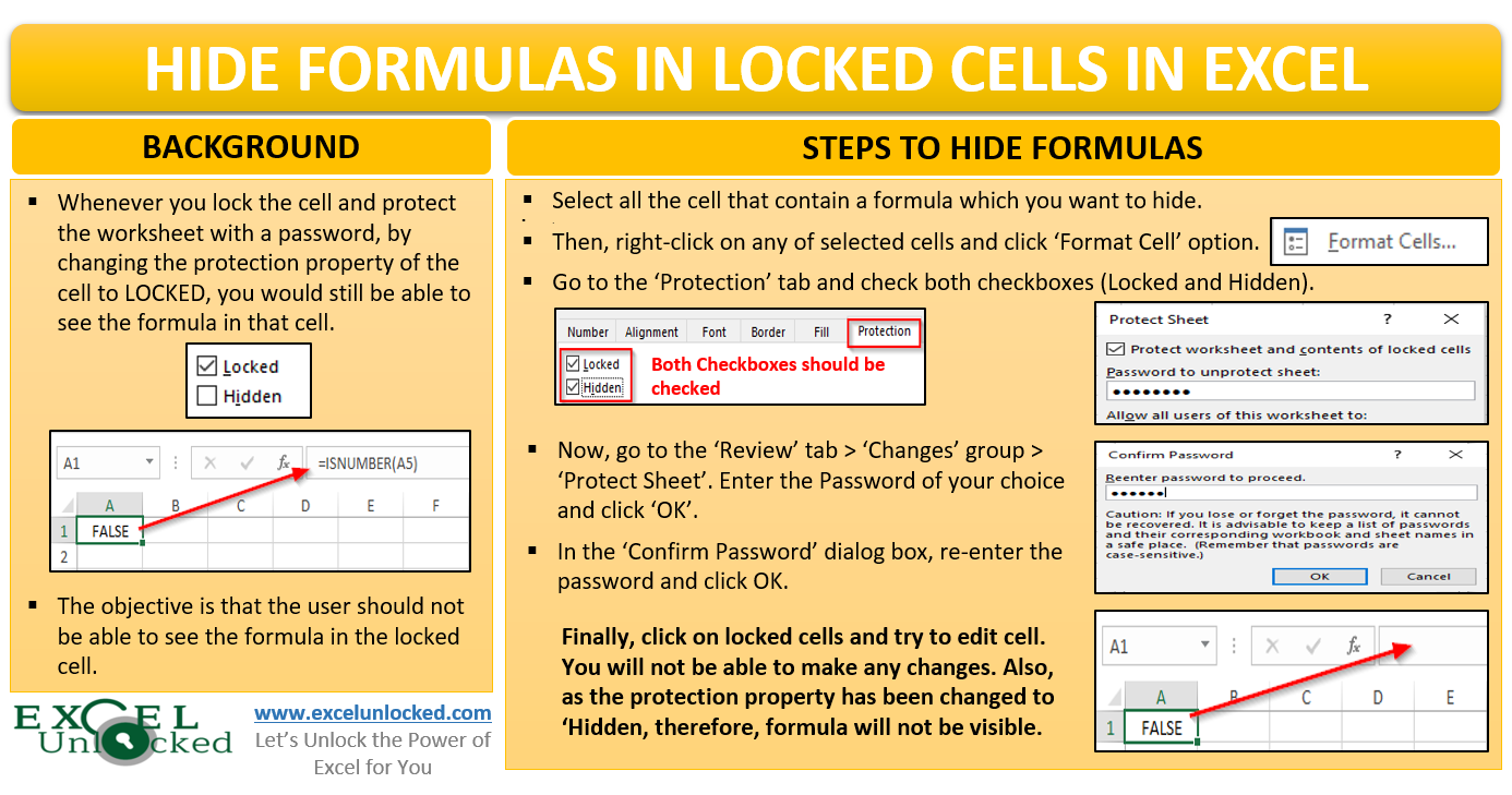
In the previous blog, we learned how to lock the cells in Excel. In continuation, in this blog, we would unlock the technique to hide the formula in locked cells Excel. Once you lock any cell in Excel, and if that cell contains any formula, then the formula is visible in the Formula bar in Excel. We can, however, hide the formula in the locked cells so that it is not visible to the unauthorized user.

Let us now begin to learn this functionality.

Concept of Hidden Cells in Excel

Like we learned in the previous blog on “How to Lock the Cells in Excel” that all the cells in any new workbook are always having the property as locked.

Similarly, all the cells in any new workbook are not “Hidden”.

It means that when we protect the workbook or worksheet, by default the formula is visible in the formula bar in Excel.

Sample Dataset

Below is the sample dataset wherein, the sale value field contains the formula (denoting Sales Unit multiplied by Selling price) and the Total Sales value of $2,280 is the sum of Sales Value.

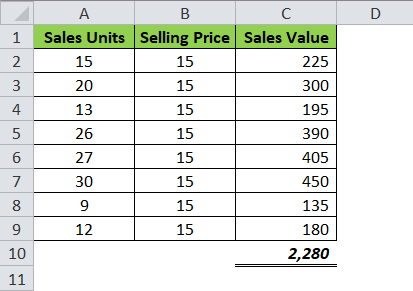
Now we wish to protect the worksheet in such a way that users of this worksheet should not be able to make any changes in column C (Sales Value). Also, the formulas entered in column C should not be visible. 

Where To Find “Hidden” Option

Follow the below procedure to navigate to the hidden property of any cell in Excel

Right-click on any of the cells. Select the option “Format Cells” from the list of available options. 

The “Format Cell” dialog box would open. Go to the “Protection” tab. There you would find the “Hidden” option.

When this option is ticked/checked, excel hides the formula in that cell when the worksheet is protected.

Hide Formula In Locked or Protected Cells

To hide the formula in the protected cell, the first step is to unlock all the cells other than those which we want to lock.

To achieve the same, follow our previous blog on “How to Lock The Cells in Excel“.

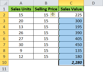
Select the formula bearing cells.

Open the “Format Cell” dialog box and click on the ‘Protection’ tab.

Tick both the checkboxes – Locked and Hidden.

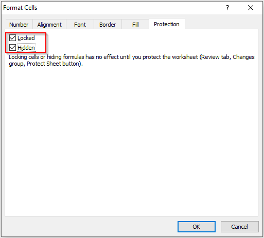
With this, we are instructing excel to lock the selected cells and also hide the formula in these locked cells when the worksheet is protected.

Now protect the worksheet with a password using the below path.

Under the ribbon bar options, click on “Review” where you would find the option called “Protect Sheet”.

As soon as you click on this option, the “Protect Sheet” dialog would open.

Enter the password of your choice in the “Password to Protect Worksheet” section of this dialog box.

Now press the “OK” button.

Re-enter the password in the next dialog box and click on ‘OK’.

This completes all the required steps.

Let us now test this functionality. Click on any cell in column C of the dataset and check the Formula Bar.

You would notice that Excel does not show the formula. The formula is not visible in the formula bar.

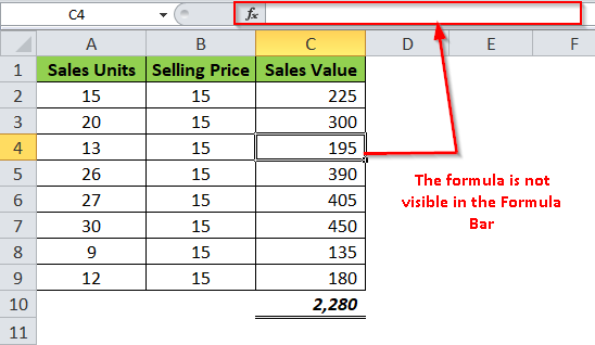
Try to edit the values in any of the cells in column C. Excel would not allow you to edit those cells as the cells are locked.

Similarly, if you try to edit any of the cells other than the cells in column C, excel would allow you to edit those cells, as the protection settings of those cells in “Unlocked”.

This brings us to the end of this blog. Share your view and comments in the comment box below.