How to Lock the Cells containing Formulas in Excel?

Today, we are going to learn a beneficial thing which is to lock the cells containing Formulas in a workbook so that no co-worker or employee can edit the important formulas that must not be changed for the workbook to perform its intended calculations perfectly.

So let us begin learning.

How to Lock the Cells Containing Formulas?

Let us suppose we have the following workbook containing certain calculations as follows.

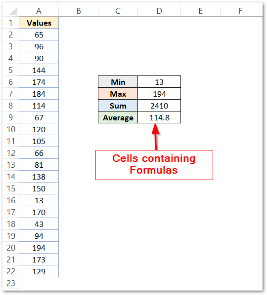
We want to lock these cells so that no one could accidentally make changes to these formulas. To protect these cells from being updated, we need to both lock as well as protect the cells of the worksheet.

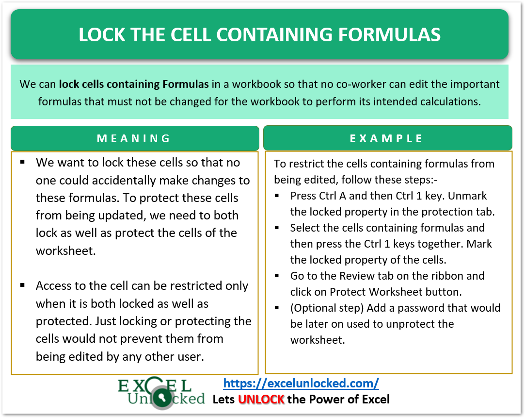
Access to the cell can be restricted only when it is both locked as well as protected. Just locking or protecting the cells would not prevent them from being edited by any other user.

By default, all the cells are locked, and we can obviously make changes to them because they are not protected. We would start by unlocking all the cells.

You can have the practice workbook to learn as well as perform these steps while reading the article.

Step 1 – Locking Only the Cells that Contain Formulas

We would start by unlocking all the cells, then locking only those cells that contain formulas.

• Press Ctrl and A keys together to select all the worksheet cells.
• Press Ctrl and 1 keys together to open the Format Cells Dialog Box.
• Go to the Protection tab and unmark the locked property of the cells.

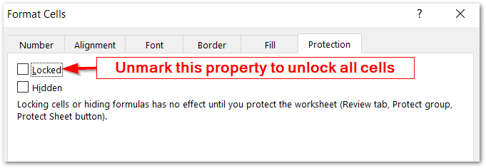
• Now select the range D6:D10 that contains formulas.
• (optional step) If the formulas are scattered across the spreadsheet, press the F5 key and click on the Special button. Click on Formulas in Go to Special dialog box and click Ok. This selects all the cells containing formulas in the current worksheet.
• Hold the Ctrl key and then press 1. Mark the Locked Property of cells in the Protection tab in the Format Cells Dialog box.

Step 2 – Protecting the Worksheet

To protect the worksheet, follow these steps.

• Go to the Review tab on the ribbon.
• In the Protect Group, click on the protect worksheet button.
• This opens the Protect Sheet dialog box. You can add a password to unprotect the worksheet thereafter. Adding a password is an optional step. Be careful while adding a password as it would be nonrecoverable. It is advisable to save a list of your passwords.

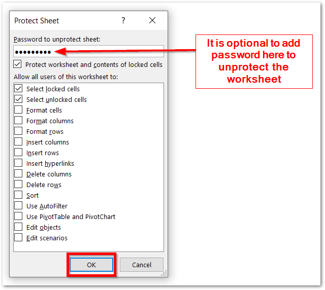
This protects the entire worksheet. The cells containing formulas were being locked as well as protected now, we would now be unable to edit the range D6:D10 whereas the other cells can be edited as they are only protected and not locked.

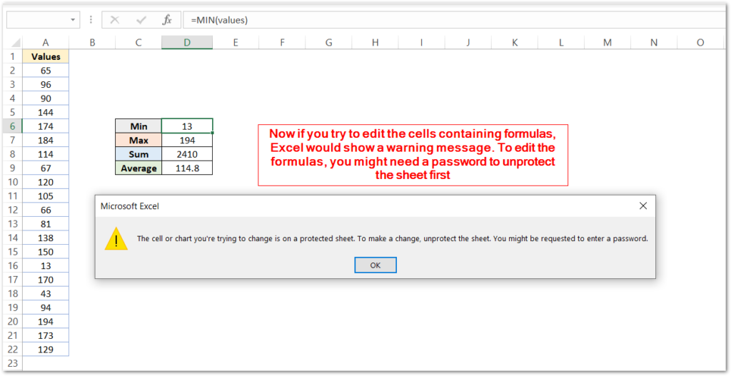
Locking and Hiding the Formula used

We have successfully locked and restricted access to edit the formulas in the spreadsheet, but the formulas are still visible in the formula bar.

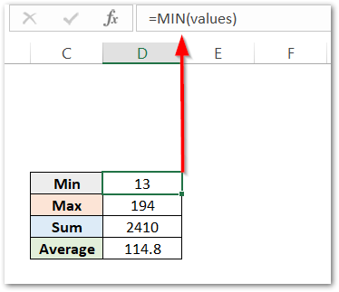
We can hide this formula in the formula bar, lock and protect the cells to restrict access to edit the formulas. To do so, we need to first unprotect the worksheet.

Unprotecting the Worksheet

To unprotect the worksheet, follow these steps:-

• Go to the Review tab on the ribbon.
• Click on Unprotect Worksheet button. You must enter a password to unprotect if you had the one while protecting the worksheet. ( We used the password as- Excelunlocked )

Hiding and Restricting the Right to Edit Formulas

now we can perform the remaining steps:-

• Select the range D6:D10 that contains formulas.
• Press Ctrl 1 key and then go to the protection tab.
• Mark the hidden property. ( make sure that the locked property is also marked )
• Again protect the worksheet from the review tab.

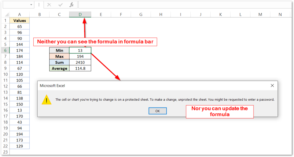
This time, we have restricted access to edit the formulas, as well as no one, would know the formulas used to get the formula result through the formula bar.

This brings us to the end of the blog. Thank you for reading.