How to Lock and Protect the Cells in Excel

Sometimes you may want that data that you have entered into your excel worksheet should not be changed by anybody. To do the same, excel has provided the functionality to lock the cells that you want should not be changed. There are multiple ways by which you can lock the cells.

Basics About Locked Cells in Excel

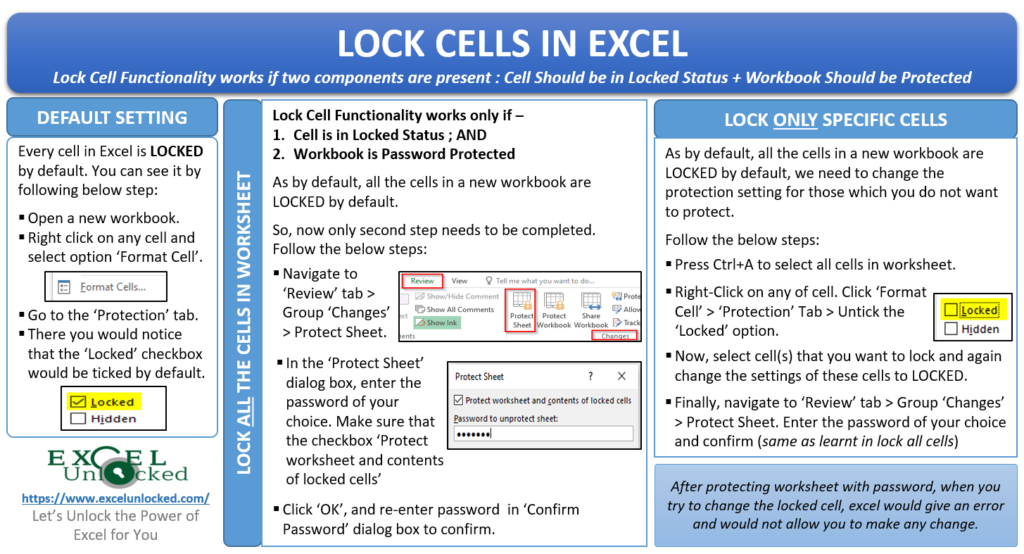
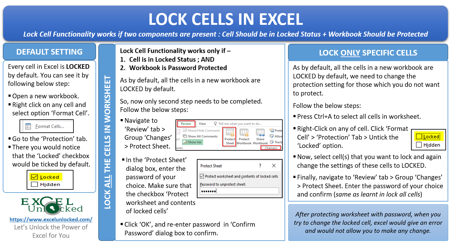
Before you go through this blog, it is important to note that every cell in Excel is by default ‘locked’.

However, this does not work until you protect the workbook.

It means that in order to completely lock the cells, two components work together. One is that the cell should be in locked status and the other one is that the excel workbook/worksheet should be protected.

Open any new workbook, right-click on any of the cells. Select the option “Format Cells” to open the dialog box “Format Cell”.

Now, go to the “Protection” tab.

In the “Protection” tab, you would notice that there are two checkboxes. One is for “Locked” and the other one is for “Hidden”.

By default, the checkbox “Locked” is ticked. It means that all the cells are by default locked in any new workbook,

Now its time to learn different methods to lock cells in Excel. Let us now begin.

Locking All Cells in a Worksheet

As mentioned above, there are two settings that are mandatory to lock any cell in Excel. The first one is that the protection status of the cell should be locked and the other one is that the workbook/worksheet should be protected.

As we know that by default, all the cells in Excel a new workbook is always locked. So now we need to perform only the second step.

Follow the below procedure to lock all the cells.

Under the ribbon options, click on the tab “Review”. In the group “Changes”, click on the option “Protect Sheet” to protect only the active sheet and select the option “Protect Workbook” to protect an entire workbook.

In this blog, we would only protect the cells in the active sheet.

As a result, the “Protect Sheet” dialog box would appear.

Now, enter the password of your choice in the “Password to Protect Worksheet” section of this dialog box.

In the “Allow all users of this worksheet to:” section of this dialog box, select the options that a user can do even in the protected worksheets.

By default, you would be able to click and select the locked as well as unlocked cells.

Now press the “OK” button.

The ‘Confirm Password’ dialog box would appear where you need to re-enter the password. Once, you have entered the password again, click on the button “OK”.

Now, try making changes in any of the cells in the worksheet. What did you notice?

You would see that every time you try to change the cell, it opens the below error window.

Also, many of the options on the ribbon are disabled and greyed out.

Lock Only Some Specific Cells

In the above section, we learned how to lock all the cells in the Excel worksheet. To lock only specific cells:

First, select the entire worksheet. To select the entire worksheet, click on any other cells in the worksheet and press Ctrl + A on your keyboard. Or you can instead click on the Select All button on the top-left of the worksheet.

Now, right-click on any of the cells and select the option “Format Cells”. Then, navigate to the tab – “Protection”.

Now uncheck the “Locked” checkbox to release the lock settings of all the selected cells and press the “OK” key on your keyboard.

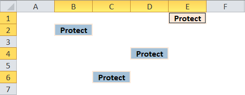
The next step is to change the protection property of only those cells that we wish to protect.

Select the cells that you wish to protect. To select the multiple cells, press the “Ctrl” key on your keyboard and click on each of those cells.

Again go to the “Format Cell” dialog box > “Protection” tab, check the “Locked” checkbox.

Under the “Review” tab, click on the option “Protect Sheet” to protect the active sheet.

The “Protect Sheet” box would pop out on your screen.

Enter the password of your choice in the “Password to Protect Worksheet” section of this dialog box and click ‘OK’.

Re-enter the password in the ‘Confirm Password’ dialog box and then click on the ‘OK’ button to exit.

Finally, let us test this. Try to edit any of the worksheet cells other than the protected one. You would notice that you are able to edit those cells.

Now, try to edit the protected cells. The excel would not allow you to make the changes and would prompt the following message.

This brings us to the end of this blog.