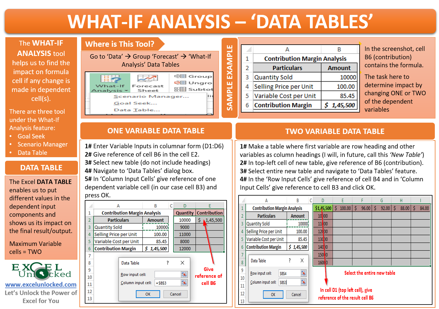
In our previous blogs, we learned about two of the What-If Analysis features in Excel – Goal Seek and Scenario Manager. In this blog, we would unlock the third and the last tool called Data Table Feature of Excel What-If Analysis. Like the other two, this feature also enables us to make the forecast. The Data Table What-If Analysis excel feature assists us to determine the impact on the result if any change is made in the dependent variable components.
Let us take one simple example to understand this functionality.
Data Table – Example
You are in the forecast and budgeting department in an organization and you use Excel as a utility software for performing your tasks. You are in the current in the process of preparing the contribution analysis budgeting tool for your manager’s usage.
Below is the screenshot of the current quarter’s contribution margin.
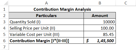
As you can see that the contribution margin (cell B6) contains the formula and is dependent on the other three variables (viz. Quantity sold, selling price, and variable cost per unit). The contribution margin is what is the final result and the other three are called the dependent variable components.
Now, suppose you want to analyze how the change in the dependent variables impact the contribution margin. You can perform the same by either using the Scenario Manager tool or the data table feature. The scenario manager feature has already been covered in our previous blog.
Also Read: What-If Analysis – Scenario Manager in Excel
In this blog, we would learn to use the data table to achieve the desired objective.
Basics About Excel Data Table
Just like the other two What-If Analysis Tools, the Excel Data table feature also helps us to do forecasting. It enables us to put different values in the dependent input components and shows us its impact on the final result/output.
The example provided in the above section is a simple one, just to make you understand the functionality. You can use the what-if analysis tools with complex formula structure for your performing the budgeting/forecasting.
Unlike the scenario manager tool, where you can create scenarios with 32 variable components, the data table can be used when you want to analyze the impact on the formula cell by changing a maximum up to TWO variable components.
In the upcoming sections of this blog, you would learn both – one variable and two variables data table creation and many more related functions.
Also Read: What-If Analysis – Goal Seek in Excel
It is important to note that the ‘Data Table’ should not be confused with ‘Excel Tables’. Excel Tables are normal tables with few additional advantages.
Let us now begin.
Where Would You Find This Feature?
Navigate to the following path to reach to this tool: Data tab > Forecast Tool > What-If Analysis button > Data Table.

Creating a One-Variable Data Table
The one variable data table allows you to see the impact on the result cell by changing one of the variable input cells.
Follow the below steps:
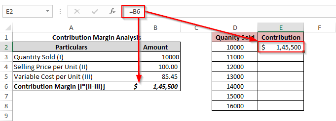
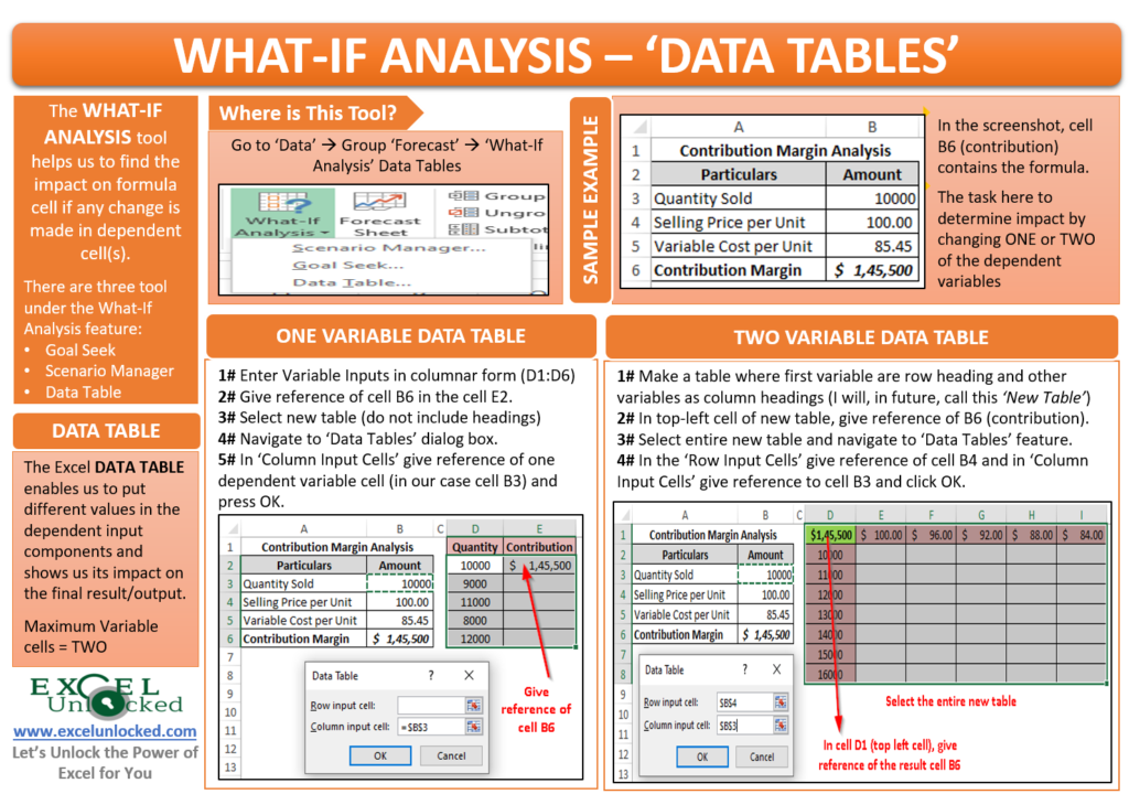
Enter the variable input values for which you want to do result analysis in either column or row. Firstly, we would learn to create a data table using the column-oriented tool. Therefore, I have put the variable input values in the form of a column.
In the adjacent cell, we want to have the resultant contribution amount. So, give the reference of the cell B6 in this adjacent cell.
Refer to the screenshot below:
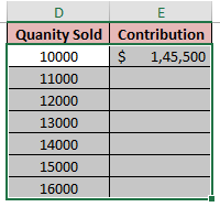
Now, select the data range including all the cells except the heading cells (in our example range D2:E8)
Navigate to the Data Table tool (as shown in the above section), and the ‘Data Table’ dialog box would pop out on your screen.
Now, click on the ‘Column Input Cell’ (As the quantities sold are in a column form) and give reference to the cell B3 in the original table. Cell B3 represents the variable Quantity Sold.
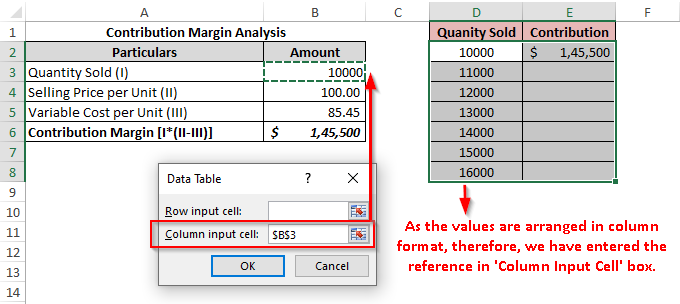
Finally, click on the ‘OK’ button and as a result, you would notice that the excel fills the contribution column (Column E) with the contribution amount based on the formula.

You can even arrange the resultant table in the row orientation. In that case, the only change is that you need to enter the reference formula in ‘Row Input Cell’ instead of the ‘Column Input Cell’.
Refer to the below screenshot:

The result would be as under:

Creating A Two-Variable Data Table
The two-variable data table helps to determine the change in the formula cell when two dependent variables change simultaneously.
In the same example, let us understand the impact on the contribution with a simultaneous change in the quantity sold and selling price per unit, keeping the variable cost per unit as a constant value of $85.45 per unit.
Follow the below steps to achieve the same:
Where you want to create a two-variable data table, you need to put one variable as the table row and another as the table columns.
I have put the column headings as the quantity sold and row headings are selling price per unit.
Then give reference to the contribution margin cell from the original table (cell B6) in this top-left cell of this newly created table as highlighted in the screenshot below:

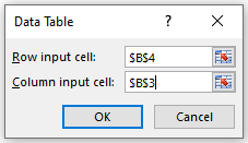
Firstly, select the entire table from D1 to I8 and then open the ‘Data Table’ dialog box.
In the section, ‘Row Input Cell’ select the cell B4 from the original table. This represents the row heading in the newly created table). Similarly, in section, ‘Column Input Cell’, select cell B3 from the original table, which represents the column headings in the new table.
As soon as you click on the ‘OK’ button, you would notice that the excel fills the blank cell s in this newly created table with the appropriate values. Refer to the screenshot below:
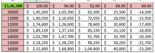
Therefore, we can see that if we sell 14,000 units at $96 each, then we would earn a contribution margin of $ 1,47,700.
This brings us to the end of this section.
How to Delete A Table
Before starting with deleting the data table, let us perform one activity. Select a cell in the data table then use your keyboard and press the ‘Delete’ key.
What did you notice? Did the excel allow you to delete the individual cell value in the data table?
The answer is NO !!
The Excel pops out a message dialog box. Refer to the screenshot below:
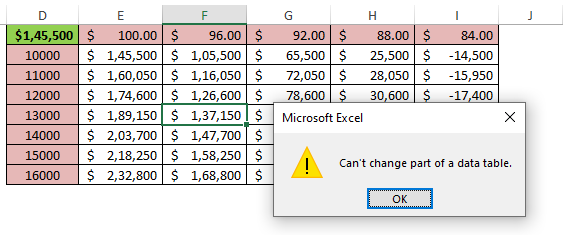
However, when you would try to delete the entire table, the excel would allow. Just, select the entire table and use your keyboard to ‘Delete’.
As a result, Excel would allow you to delete the values.
This brings us to the end of this blog. Share your views and comments in the comment section below.

