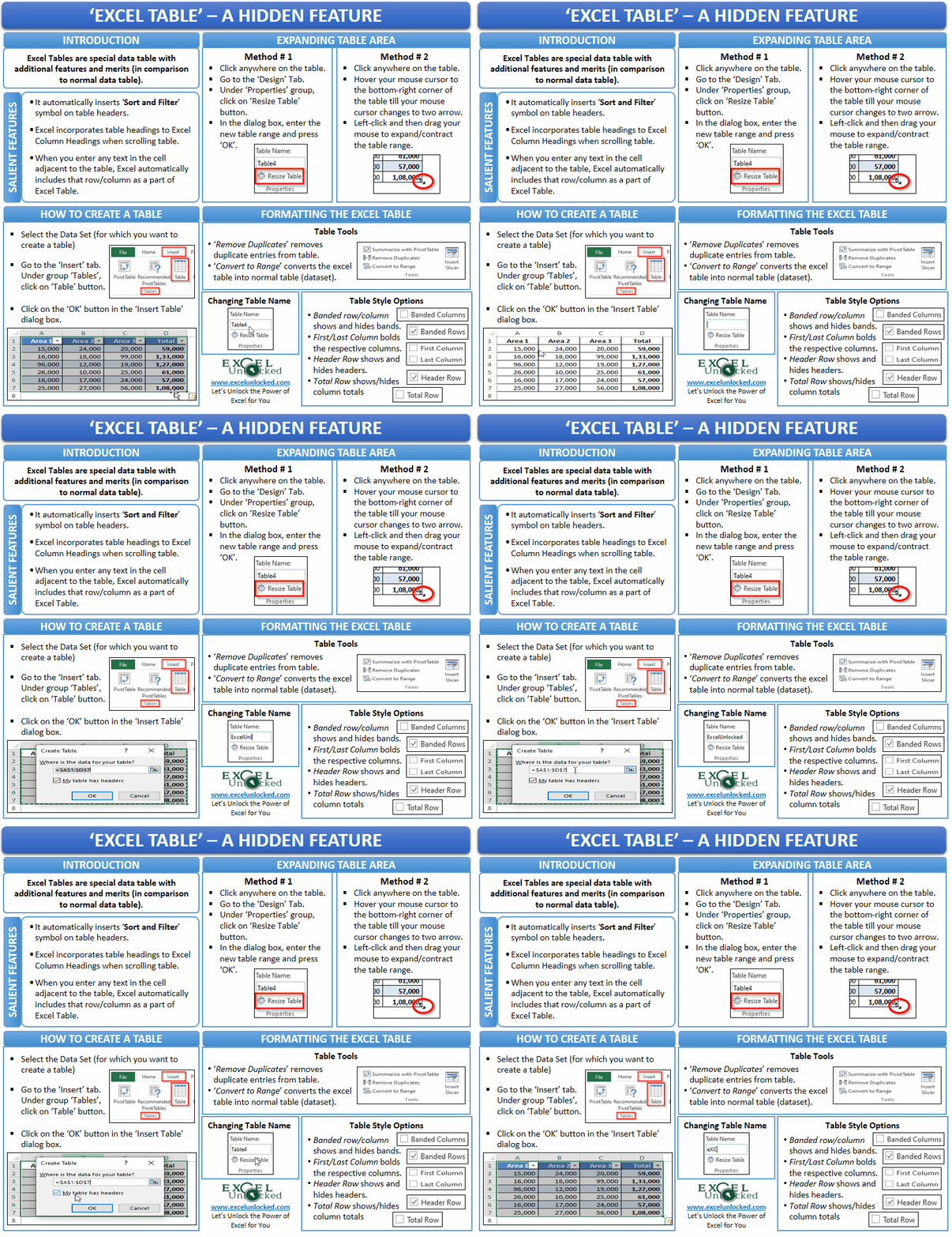
A Table in Excel is an Amazing feature provided in Microsoft Excel. It has a bunch of features that make tasks in Excel very easy. When you convert your Excel dataset in a tabular format, you can quickly analyze your data. There are a lot of unknown merits of this functionality. In this blog, we would learn everything about table functionality in Excel.
Creating a Table in Excel
If you have data in Excel which is not a table form, you can easily convert that data into the tabular form using the below simple steps.
Firstly, select the complete dataset.

Then, in the ribbon bar, click on the tab ‘Insert’. There you would find a button ‘Table’ in the group ‘Tables’. Refer to the image below:

As soon as you click on the ‘Table’ button, a small ‘Create Table’ dialog box would pop up. In this dialog box, you can find two options.
The first one is the input box where would notice that Excel automatically inserted the selected table range.
And the second one checkbox to instruct excel if your data table contains a header row or not. Check this checkbox, if your table has headers in it. As my table has a header row, therefore, I have ticked this option.
Uncheck that option, if your excel table does not have any header.
Then, click on the ‘OK’ button to activate the options.

As soon as you click on the OK button, your dataset would get converted into a table format as shown in the screenshot below:

An Excel Table distinct from the Normal dataset table on the following basis.
An Excel Table would have alternate colored rows (the banded rows).
It would also have a different header row color. As you can see our original dataset (normal table) does not have any fill color, but the excel table (converted) has its header row in a blue fill color.
Also, an Excel Table would automatically insert the filter option on the header rows.
Salient Features
As mentioned in the introduction of this blog, there are many additional amazing features of an Excel table vis-a-vis a normal dataset in Excel. Let us go through each of these merits one by one.
Also Read: 2 Ways to Use Transpose Function in Excel
The most important feature of this is that Excel automatically puts ‘sort and filter’ buttons on the header row.

Another amazing thing that you would notice is that whenever you scroll down your data, Excel would insert the headers in the Excel column headers. This would function only when the table is selected. Refer to the below demonstration below:

The next feature is that when you enter anything in the cell adjacent to the current selection, excel would automatically expand the area and include this new data.

How to Expand the Table Selection Area?
As mentioned in the ‘Salient Features’ section of this blog, the Excel would automatically expand the selection area, when you enter anything in the adjacent cell.
However, apart from this, there are two more ways to do it.
The first one is by using the ‘Resize Table’ dialog box and the second one is by using mouse drag and drop functionality.
Let us learn each of these ways one by one.
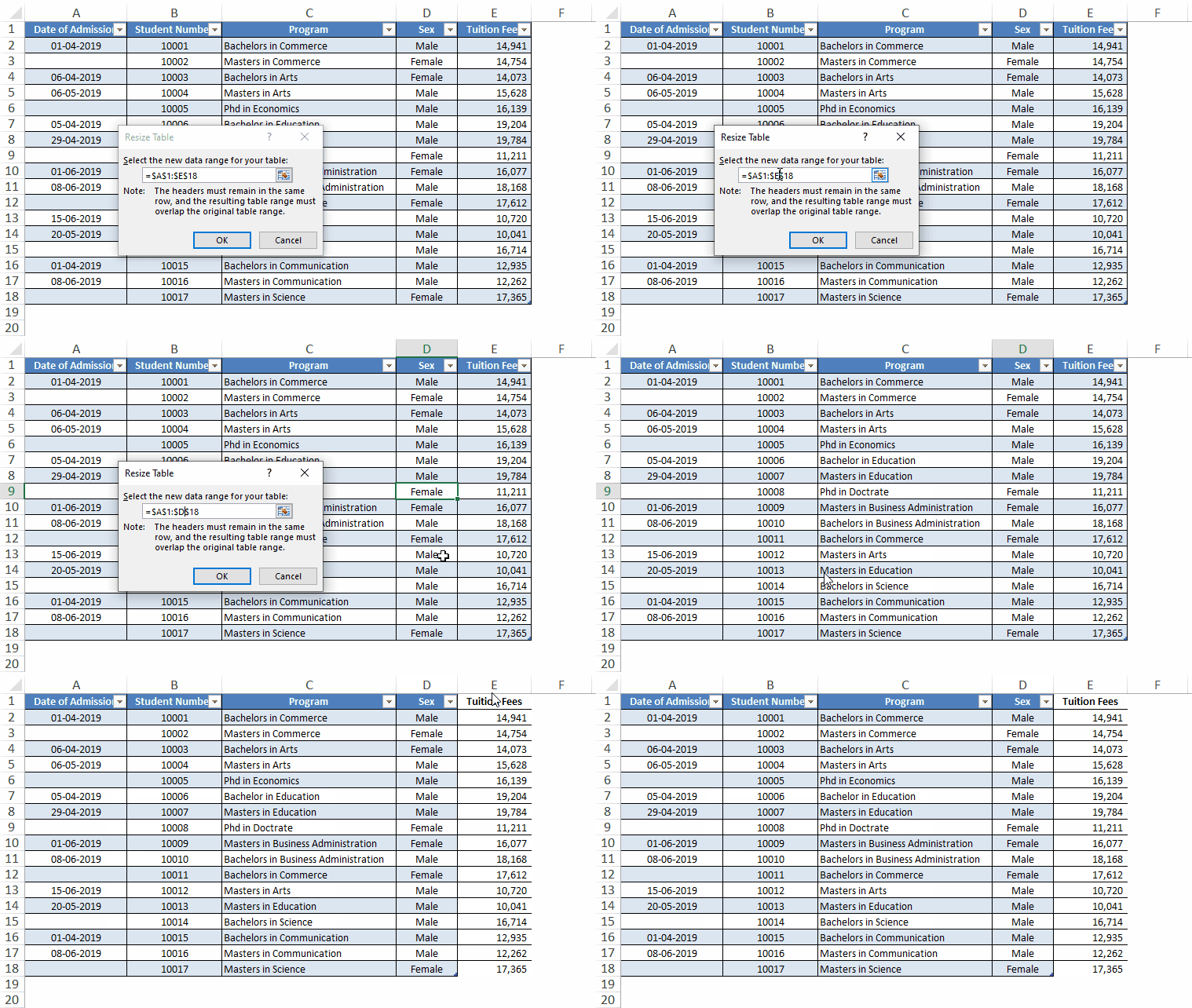
Firstly, click inside the Excel Table. You would see that the ‘Design’ tab automatically appears on the Excel ribbon bar.
Click on this tab ‘Design’. Under the group ‘Properties’ click on the button ‘Resize Table’.

The ‘Resize Table’ dialog box appears. In the input box of the dialog box, enter the new table range and click on the ‘OK’ button.

Another way is to use the mouse drag and drop feature. Click anywhere on the table and hover your mouse cursor to the bottom-right corner of the excel table.
As soon as you see the two-faced arrow symbol, left-click on your mouse and drag it to expand or contract the range.

Formatting The Excel Table
To format an Excel Table, click anywhere on the table and you would notice that the ‘Design’ tab appears on the ribbon bar. In this tab, there are variety of options available to format the Excel Table.


Table Name: Here you can change the name of the table as per your choice. Giving a name to a table is very useful for giving reference to a table in Excel.
Resize Table: This option helps to change the expand or contract the table area (as discussed in the above section).

Summarize with Pivot Table: This option generates a pivot table.
Remove Duplicates: This option removes duplicate values and only keeps the unique values.
Convert to Range: This option converts back the Excel Table into a normal dataset table.
Insert Slicer: This option inserts a slicer. (In detail below)

External Table Data: This group contains options to export and refresh the table data.

Header Row: This option helps to show or hide the header row of the table.
Total Row: This option helps to insert and disable the total of columns at the end of this table.
Banded Rows: This option shows and removes the fill colors from the alternate rows.
Banded Columns: This option shows and removes the fill colors from alternate columns. (Generally not checked)
First Column: This option, if checked, bolds the text in the first column.
Last Column: This option, if checked, bolds the last column in the last column.
Filter Button: This option shows and hides the filter button from the table headers.
However, default excel settings under this group are as below:

Table Style: This section of the ‘Design’ tab helps us to change the style of the table from the available options. This option enables you to create your own style as well.

Using Slicers in Excel Table
The Excel Slicers are very interactive tools that helps us to filter the data quickly on the click of a button.
The Excel Table Slicers are introduced in Excel 2013 version.
Let us now learn about Excel Slicers and its functionality.
Inserting Excel Table Slicers
Follow the below steps to insert a Slicer.
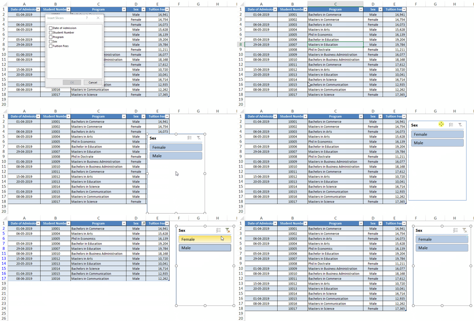
Click on any cell in the Table. The ‘Design’ tab would appear on the ribbon bar.
Go to this new tab and click on the button ‘Insert Slicer’ under the group ‘Tools’.

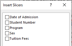
The ‘Insert Slicers’ dialog box would appear. In this dialog box, you would notice that the table headers would appear (with checkboxes on its left).

Check the header checkbox(es) to which you want to add the filter and click on ‘OK’ button
You would notice an interactive box would appear for the selected checkbox(es).
Now, you can click on the buttons in the slicer to filter the data.

This brings us to the end of this blog. Share your views and comments in the comments section below.
