In this tutorial, we would learn one of the most important features of Excel that allows you to organize your Excel data table. The feature about which I am taking is the “Sorting” feature of Excel. There are multiple ways in which you can sort a table or data in Excel.
Let us now get an insight into what this tutorial aims at achieving.
In this tutorial, you would learn how to sort the data table by a single column and by multiple columns. You would also learn how to change the orientation of sorting. With this technique, you would be able to sort the data table from left to right.
Prepare the below sample dataset table:
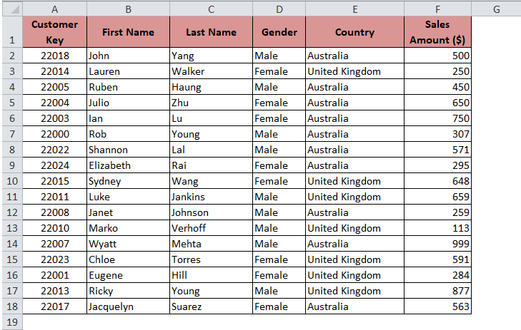
Let us now begin with each of these sorting features.
Sort by Single Column
In this section of this blog, you would learn how to sort by a single column in an Excel table. You want to sort your Excel dataset table in ascending order based on the First name.
It is a simple two stepped procedure.
In order to sort the dataset based on the first name (Column B), select any cell in column B of the dataset.
Also Read: Sort Rows in Excel – Sort from Left to Right
Under the ‘Data’ tab, in the “Sort & Filter” group, click on the “Sort A to Z” button as highlighted in the screenshot below:

As a result, the dataset table gets sorted in ascending order (A to Z) based on the First Name.
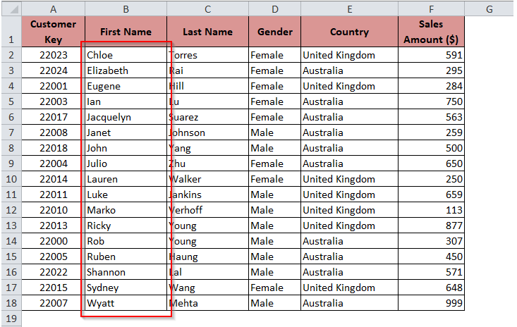
Now suppose you want to sort the data in the descending order (Z to A) based on the Country, you need to first select any cell on column E (Country) and then click on the “Sort Z to A” button in the “Data” tab.

Note that using the “Sort A to Z” and “Sort Z to A” buttons, you can only sort the dataset table based on a single column.
Sort by Multiple Columns
Suppose you want to sort your dataset in a way that the country names are in ascending order and the highest sales value should come first.
Follow the below steps to sort by multiple columns:
Select any cell in the dataset table.
Under the ‘Data’ tab, in the “Data & Filter” group, select the “Sort” button as shown in the screenshot below :

The “Sort” dialog box would open.
Step 3: In the “Sort” dialog box, check the checkbox “My data has headers” checkbox is checked as highlighted in the screenshot below:
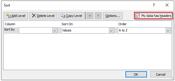
By checking this option, we are telling excel that the dataset table has the first row (Row 1) as the heading row.
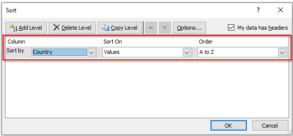
As we want to first sort the dataset by “Country”, select the option “Country” from the drop-down list in the “Column” heading of this dialog box.
The “Sort On” option would be “Values”. The “Order” of sorting shall be selected as “A to Z” for sorting in ascending order.
The above settings in step 4 would look like this :
Now to further sort the table based on the sales amount, we need to add a new level to the sorting settings.
To add an additional sorting, you have an “Add Level” button. Click on this button.
This would add a new level just below the first level of sorting as highlighted in the screenshot below :
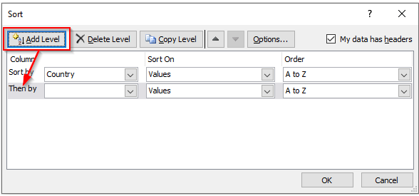
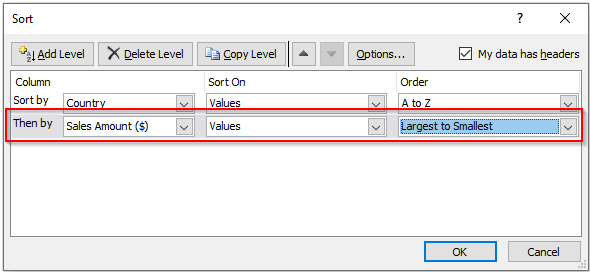
Make the settings on the second level of sorting.
The column heading would be “Sales Amount ($). And the sort order would be “Largest to Smallest” as we want to sort this list in descending order. Finally, click ‘OK’.
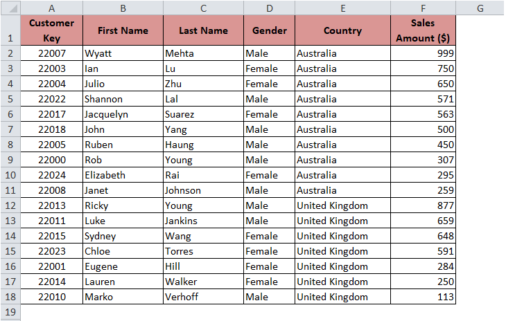
You would notice that the dataset table sorts in the ascending order based on the “Country” (Australia comes first and then the United Kingdom).
Also, the ‘Sales amount gets sorted from Z to A.
Changing Orientation of Sorting in Excel Table
Generally, tables in Excel have headings on the top of the table.
However, many a time, you may have a table with its headings on left.

In order to sort such tables, it is not possible with the technique explained about.
We need to make some changes in the sort settings. Follow the steps to achieve the same:
Select any of the cells inside the table.
Under the ‘Data’ tab, in the “Data & Filter” group, select the “Sort” button as shown in the screenshot below :

As soon as you click on the ‘Sort’ button, the “Sort” dialog box would pop out.
Here, click on the button “Options”.
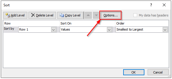
The “Sort Options” dialog box would appear on your screen.
Select the radio button “Sort left to right” and click on the “OK” button.
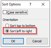
Now you are ready for sorting the data in Excel.
Firstly, select the dataset. But, do not includes the headings (A1:A3) in the selection.

Under the heading “Row”, select the row number by which you want to sort your data.
Suppose I want to sort my data by “Customer key”, i.e. row 1, therefore, select the option “Row 1” from the drop-down menu.
In the “Sort On” heading, select the option “Values” from the drop-down options.
And in the “Order” heading, select the option “Smallest to Largest” to sort the data in ascending order or “Largest to Smallest” to sort the list in descending order.
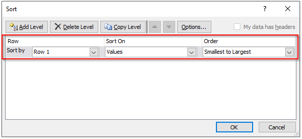
As soon as you click on the “OK” button, you would notice that the entire table is now sorted based on the “Customer Key”.
This brings us to the end of this blog. Share your views, reviews, and comments in the comment section below.

