Do you know how to create a dependent drop-down list in an Excel worksheet? At the end of this blog, you would be able to create a dependent drop-down list in which the drop-down list in one cell depends on the value in another cell. This is also known as a Conditional drop-down list.
It means, if the value in one cell is changed, the drop-down list of the other cell would accordingly change.
Before going through this tutorial, revisit our earlier blog on “How to Create a Drop-Down List in Excel“
Now let us understand what this blog aims at achieving.
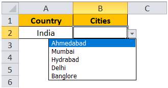
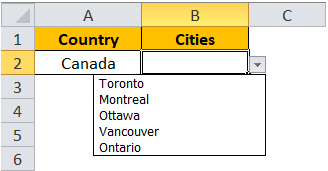
As you can see from the below screenshots, when the value in cell A2 is “India”, the drop-down list in cell B3 contains the names of cities in India. And where the country is changed in cell A3 to “Canada”, the drop-down list in cell B3 changed accordingly. Now it contains only the names of cities in “Canada”.
Let us unlock this technique. The entire process would be done in 3 steps :
- Creating a Drop-Down List for Countries
- Naming the Cell Range
Creating a Drop-Down List for Countries
Step 1 : Make the following sample table (consisting of the list cities in countries India and Canada) in an Excel worksheet.
Also Read: How to Create a Drop-Down List in Excel
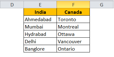
Step 2 : Select the cell where you want the first drop-down list. In our case, we would select cell A2 depicting the country name.

Step 3 : Go to be “Data” tab. Under the “Data Tools” group, select the option “Data Validation”.

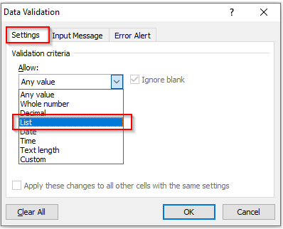
This would open the “Data Validation” dialog box as shown in the screenshot below :
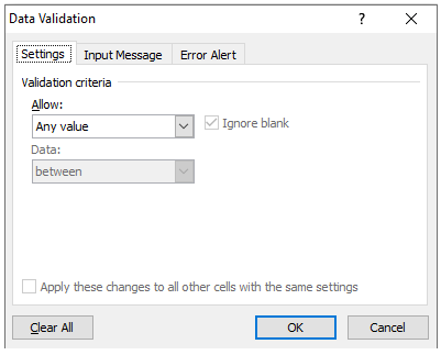
Step 4 : Under the “Validation Criteria”, select the option “Lists” from the drop-down options.
Step 5 : The “Source” field would appear in the dialog box.
Check the “In-cell dropdown” option. If it is unchecked, the drop-down functionality will not work.
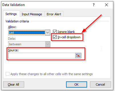
Step 6 : Click on the button adjacent to the ‘Source’ field and select the range of cells that contain the country name as shown in the screenshot below.

And click on “Ok” button.
You would notice that the selected cell A2 now contains the drop-down list consisting of the names of countries “India” and “Canada”.
Naming the Cell Range
In order to give a name to a cell range, follow the below procedure.
Step 1 : Now, select the entire data set (including the table headings) as shown on the screenshot below :
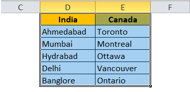
Step 2 : Go to the “Formulas” tab. Click on “Create from selection”. This is available in the group ‘Defined Names’ as highlighted in the screenshot below.

The dialog box “Create Name from Selection” would pop up. Check the “Top Row” checkbox and deselect the others as shown in the screenshot below.
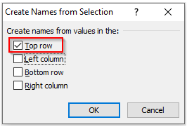
Click on the “OK” button.
This would create two name ranges. One as “India” and another “Canada”.
To verify the same, select the range of cities in “India” (cell D2:D6) and check the name box as highlighted in the screenshot below :
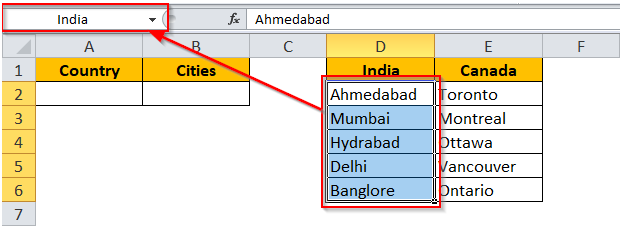
Similarly, select the cell range E2:E6, and check the name box.
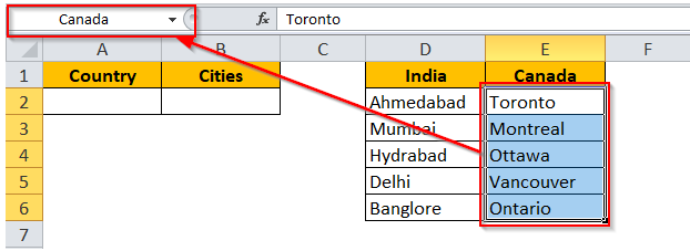
Creating Dependent Drop-Down List
Step 1 : Select the cell where you want to create a dependent list (in our case – B2). The drop-down list in cell B2 would depend on the value in cell A2
Step 2 : Go to be “Data” tab. Under the “Data Tools” group, select the option “Data Validation”.

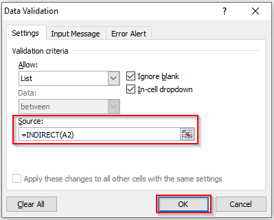
The “Data Validation” dialog box would pop up on your screen.
Step 3 : Under the “Validation Criteria”, select the option “Lists” from the drop-down options.

The “Source” field would appear in the dialog box.
Step 4 : Enter the following formula in the Source Field :
=INDIRECT(A2)
And click on “Ok” button.
This being us to the end of all the steps. Let us now test this functionality.
Select “India” from the list in cell A2. Consequently, you would notice that the drop-down list of the Cities (cell B2) would only contain the names of cities located in India.

Now change the country in cell A2 to “Canada”. Now, check the cell B2.
As a result, you would notice that now the drop-down list has updated to the cities located in Canada.

This brings us to the end of this blog. Share your view and comments in the comment section below.

