INDIRECT Function in Excel – Get Values from Reference

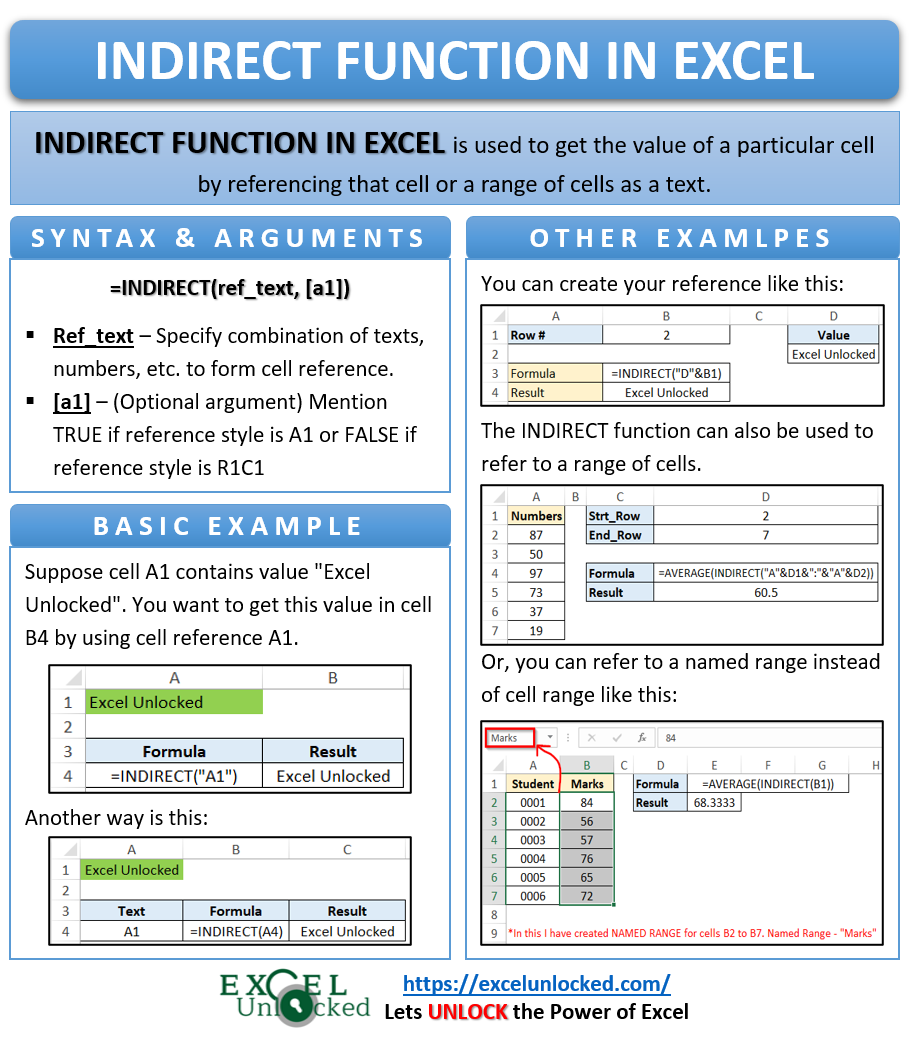
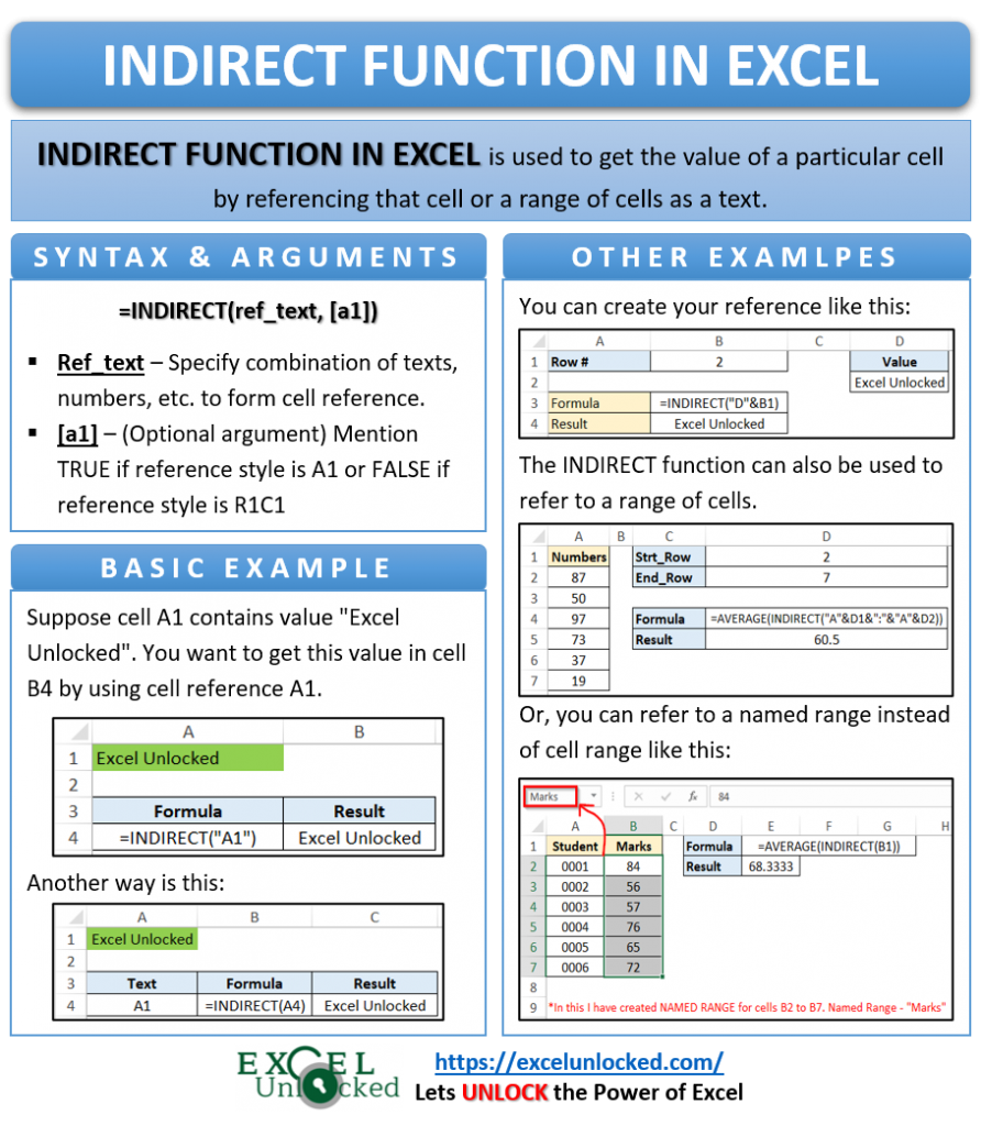
The INDIRECT function in excel is a reference excel formula which references a cell or range of cells to get its values. This blog would help you to understand bits and pieces of the excel INDIRECT formula.

At the end of this tutorial, you would have an excellent understanding of how the INDIRECT Function in excel works and how to use the INDIRECT formula in excel.

This tutorial contains a logical understanding of INDIRECT function, its syntax, arguments and some basic to advanced examples.

So, let us begin 😎

When To Use INDIRECT Function in Excel

The excel INDIRECT formula is used to get the value of a particular cell by referencing that cell or a range of cells as a text.

In simple terms, you can create or generate a formula or cell reference by using texts, numbers, exclamation marks, inverted commas, etc. And then use this cell reference to get its cell value.

Syntax and Arguments

=INDIRECT(ref_text, [a1])

The above formula has two input arguments, as explained below:

• ref_text – In this argument, specify the combination of texts, numbers, etc. to form a cell reference (text string).

• [a1] – This is a optional argument. In this argument, mention TRUE if reference style is A1 or FALSE if reference style is R1C1. If this argument is kept as blank, excel defaults it to TRUE (i.e. A1 style).

Examples on How INDIRECT Function Works in Excel

Let us deep dive into some examples of INDIRECT excel formula. In the upcoming sections of this blog, I would take you through some basic examples to understand the working of excel INDIRECT function.

1# Using Cell Reference to Get Cell Value

Suppose cell A1 contains a value “Excel Unlocked”. Now, you want to get this value in another cell by using the cell reference A1.

In that case, simply type A1 within double quotes as an INDIRECT formula input argument.

=INDIRECT(“A1”)

OR

=INDIRECT(“$A$1”)

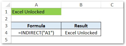
Explanation – In the above example, you would notice that the INDIRECT formula interprets the text within double quotes (i.e. A1) as a cell reference and returns the value in cell A1 – “Excel Unlocked”.

Instead of manually typing A1 in the cell, you may give it use cell reference as an input argument, as demonstrated below:

2# Creating Own Cell Reference to Get its Cell Value

Now when you have a basic understanding of how INDIRECT formula works in excel, let us now go a bit further.

Using the INDIRECT formula, you can create a cell reference and then fetch the created reference value.

Have a look at below example:

Cell D2 contains a value “Excel Unlocked”, and cell B2 contains the row number of cell D2.

You can easily get the cell value in D2 by creating the cell reference using the INDIRECT excel function.

=INDIRECT(“D”&B1)

Explanation – The text string “D” returns D and B1 returns the cell value in cell B1 which is 2. Concatenating D and 2 using an ampersand (&) results into D2. The INDIRECT function then interprets D2 as a cell reference and returns its value. It’s that simple.

3# Using Cell Range in INDIRECT Excel Function

In addition to referencing a single cell, the excel INDIRECT formula also allows you to reference to a range of consecutive cells. This consecutive cell range can then be used to perform mathematical operations like SUM, AVERAGE, and so on.

See the image below for better understanding:

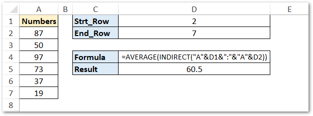
Formula Used – =AVERAGE(INDIRECT(“A”&D1&”:”&”A”&D2))

Explanation – The input argument of INDIRECT function INDIRECT(“A”&D1&”:”&”A”&D2) returns cell range A2:A7. Finally, the AVERAGE function returns the average of the numbers in cell range A2:A7. resulting in the value 60.5.

4# Creating Sheet Reference Using INDIRECT Formula in Excel

Before learning to use INDIRECT function for referencing another sheet, let us first see how excel understands the cell reference in another sheet.

• Suppose you are working in excel worksheet named ‘First’ and in this you want to reference a cell A1 of another sheet named ‘Second’. To do so, you use =Second!A1. This means that the cell and the sheet’s name are separated by an exclamation mark while referencing.

• However, if the sheet’s name contains two of more words (for e.g. – ‘Second Sheet’), then excel automatically puts the sheet name within single inverted commas like this =’Second Sheet’!A1.

Now, let us see how to work with create input argument of INDIRECT function to refer to a cell in another worksheet.

The easiest way is to give cell reference as text string within double quotes like this:

=INDIRECT(“Second!A1”)

Or,

=INDIRECT(“Second!A”&ROW())

Explanation – In the above formula the text string “Second!A” returns the text Second!A and the ROW() formula returns the row number of the active cell i.e. 1. These are then concatenated using the ampersand sign (&) to create sheet’s reference “Second!A1”.

Now, to create reference to a sheet with sheet’s name having more that one word, remember to use single inverted at the beginning and end of the sheet’s name. See the example below:

=INDIRECT(“‘Second Sheet’!A1”)

Or, if you have the sheet’s name and cell reference name in a cell then you can reference those cells instead of manually typing it. See the example below:

=INDIRECT(“‘”&B1&”‘!”&B2)

Explanation – In the above example, the “‘” returns single inverted (‘), B1 returns value in cell B1 which is ‘Second Sheet’. Similarly, “‘!” returns single inverted followed by exclamation mark (‘!) and B2 returns value in cell B2 which is ‘A1’. Concatenating all these elements result in sheet reference ‘Second Sheet’!A1.

5# Creating Sheet Reference Using Named Ranges

In addition to the above ways of referencing the cell range, you can even use the named range for accomplishing this.

See the below image and the explanation to understand how to use named ranges in INDIRECT excel formula.

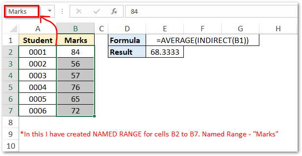
Explanation – In the above example, I have created a named range with text “Marks” to refer cell range B2:B7. The INDIRECT function with input argument B1 interprets the value in B1 i.e. “Marks” as a named range and as a result, returns the range of cells B2:B7. Finally, the AVERAGE function finds out the average of the INDIRECT function’s result (i.e. cell range B2:B7).

Using INDIRECT Function in Practical Scenario

Now when you have an overall understanding of how the excel INDIRECT formula works in different scenarios, let us consider one practical aspect of using the INDIRECT function in excel.

The named range feature of excel along with the INDIRECT function helps you to create a dependent drop-down list in excel. In this, you can use the above function to change one drop-down list value based on another drop-down list.

To learn more about this in detail, refer to the ExcelUnlocked blog on ‘How to create a dependent drop-down list in excel‘.

Thanks You 🙂