Relative Referencing in Excel – Types of References

References form the base for using the formulas and functions in excel. If one wants a good grip on excel, then they must know the correct use of references as not knowing references creates trouble a lot of time. So let’s begin learning.

What is Referencing?

With the word Referencing, we are actually meaning ‘referencing of cells’ in excel.

Question – How do you call your friends? By their name, obviously. There are 16,777,216 total cells in one excel spreadsheet. So how would you refer to a particular cell in a formula to use the cell value?

The answer is simple. One cell is made by the intersection of one row and one column. The pair of each column and each row that intersect to give one cell will provide the name of that cell.

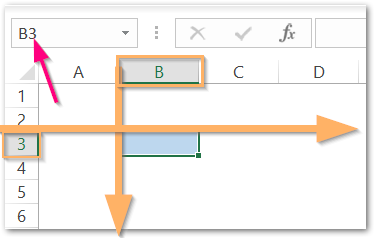
The cell highlighted in blue is named B3 as you can see in the name box pointed with a red arrow.

This is so because column B and row 3 intersection formed that cell.

So that cell will be referred to as B3.

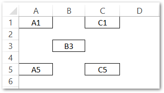
Here above are some examples, the cell name is typed into the cell.

Now, Referencing focuses on what happens to the cell in any formula, when we copy that formula to other cells. We can copy the formula by using excel fill handle tool also, but there are some keyboard shortcuts too!

Types of Referencing in Excel

There are three types of cells references in excel mentioned below:-

• Relative Referencing
• Absolute Referencing
• Mixed Referencing

All three references have their usage as per the need while we copy the formula to other cells. In this article, we will start by learning the Relative Referencing first.

What is Relative Referencing in Excel?

The word relative means the formula will relate somehow. In other words, We can say that, when we copy the formula to other cells, the formula references in the formula will update themselves as per each cell we copy the formula to.

Relative Referencing in Excel is the default referencing type. This might seem intimidating to understand but, the example is a savior.

Example 1 – Copying formula to down one cell

Let us say we have the following data:-

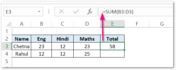
Here are two student records for marks and we have got a total for Chetna’s marks by using the SUM function in excel.

Now, go to cell E4 and press the ctrl D key.

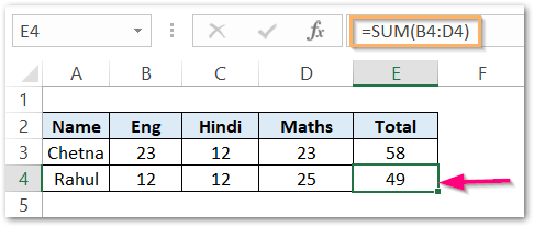
The formula has been copied to cell E4 with relative referencing. Now see the difference in the formula for both cells E3 and E4.

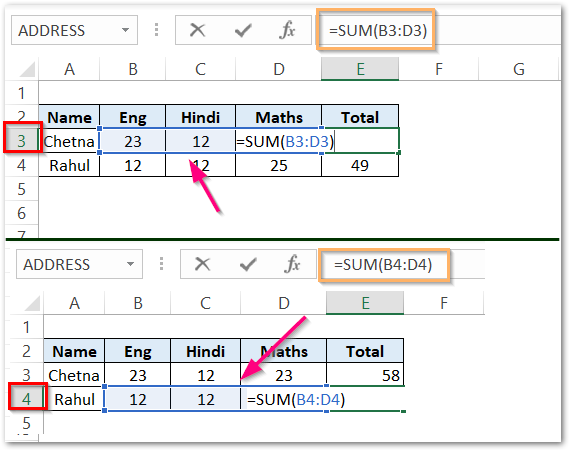
Explanation – Here for cell E3, the formula was supplied with a range of cells B3:D3. But when we copied the formula to cell E4, it changed to range B4:D4. We copied our formula, exactly one row down ( 3rd to 4th ) and the references in the formula also dropped to one row below.

Example 2 – Copying Formula to the Right

Let us say we have the following set of values:-

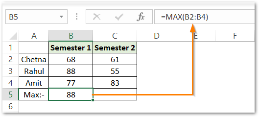
Here we have records of three students and we want to know the maximum marks for each semester’s results, for which we used the MAX Function in Excel in cell B5. We will copy this formula to cell C5 to get the max marks for the 2nd semester.

Select cell C5 and press the ctrl R key as the formula copies to the right of B5.

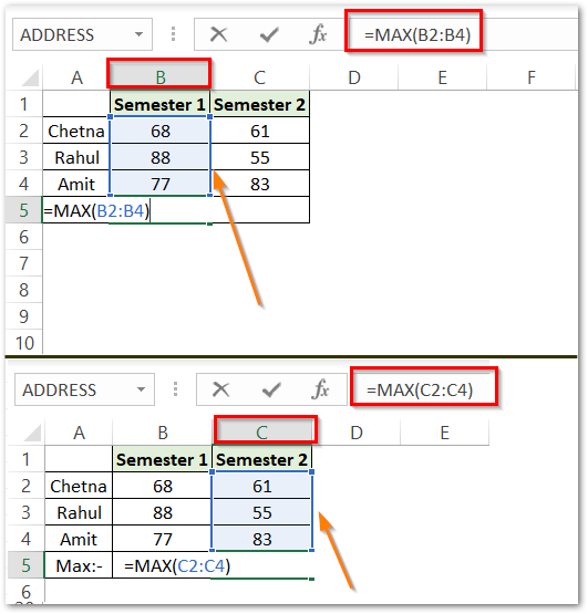
Explanation – We copied the formula from cell B5 to C5. We basically moved to one Column to the left of Column B, which is column C. The references used in cell B4 were B2:B4 and they also changed to C2:C4 ( one column to the left ).

You must extend your learning by reading the article for Absolute Referencing in Excel and Mixed Referencing.

This brings us to the end of the blog. Thank you for reading.