In the previous blog, we understood the usage of Relative Referencing. We highly recommend reading the Relative Referencing before jumping to Absolute. The second referencing type is absolute referencing in excel and no one can replace its usage with anything else!.
Let us start learning.
What is Absolute Referencing in Excel?
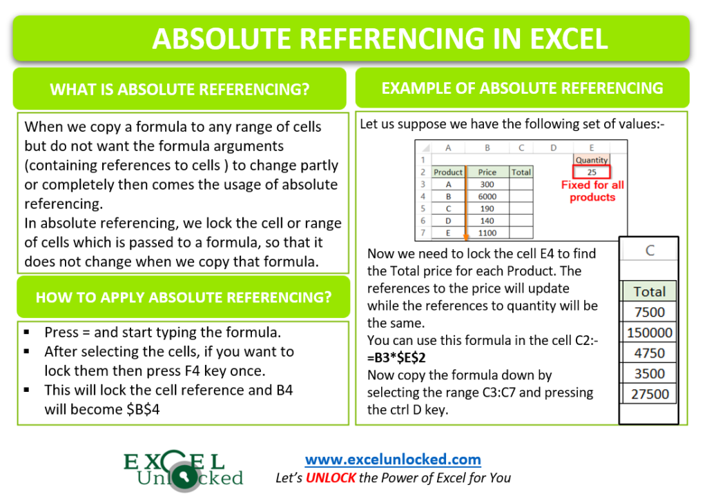
When we copy the formula to any range of cells but do not want the formula arguments (containing references to cells ) to change partly or completely then comes the usage of Absolute Referencing.
In absolute referencing, we lock the complete cell ( or range of cells ) which is passed to any formula so that it does not change when we copy that formula.
A cell forms by the intersection of rows and columns. So when We put the Dollar sign ($), it is to lock the cells by fixing both the row and column for that cell.
For example, cell B3 will become $B$3. The shortcut to apply absolute referencing while selecting the cells is to press the F4 function key after selecting the range of cells.

How to apply Absolute Referencing?
There are the following steps to use absolute referencing in excel:-
- Press = and start typing your function name. When you find that function at the top of the default function list then press the TAB key to complete the name of the function and start the brackets automatically.
- Now you need to select the range ( group of cells ) you want to supply as a function argument. To lock that range ( apply absolute referencing ) simply press the F4 Function key. This will add a $ sign to those references
- Complete your formula, now if you copy it anywhere in your worksheet, the locked cell reference wouldn’t automatically update.
Example 1 – Applying Absolute Referencing
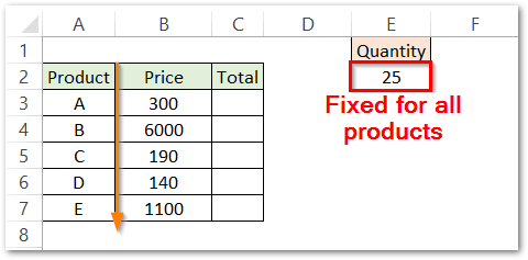
Let us suppose we have the prices of products and every product has the same quantity.

Now, the prices are different. we want to get the total bill for each product which is simple Quantity*price. Since we need to lock the quantity so:-
- Go to cell C3 and press =
- Select cell B3 and press *. Now select the cell E2. as we need to lock E2, press the F4 key. This will add the Dollar sign to cell E2 ( both Column E and Row 4 ) and make it $E$2.
- This will give the formula in cell C3 as
=B3*$E$2
Now select the range C3:C7 and press ctrl D to copy the formula down.
The formula for last cell C7 will become:-
=B7*$E$2
You can see here that the price has been updated in range C3:C7 because of Relative Referencing as per the product but the Quantity contained in cell E2 is locked as $E$2 and remains the same.

Example 2 – Using Absolute Referencing with Relative Referencing
Most of the time, absolute referencing cant be used alone in the formula itself. We need some sort part of references to change while some arguments are still locked to get the different formula results.
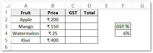
In this example, let us suppose we have the price of different fruits and the percentage of GST to add to each fruit price is constant i.e 6 %.

Now we would like to calculate the values for the GST column. We would first type the formula in cell C2.
=B2*$F$4
and you can copy the formula to the rest of the cells by simply selecting the range C2:C5 and pressing the Ctrl D key.
Press Ctrl ~ (tilde at the top left of your keyboard ) to see all your formulas in the sheet.

So you can see that Prices in the formula change while the cell F4 is locked and remain the same in all the cells in GST Column. You can press Ctrl ~ again to toggle the usage and get back to formula results.
Now use the formula in cell D2.
=B2+C2
Copy the formula down by simply pressing the ctrl D after selecting the range D2:D5.
You will see that all the GST corresponding to the fruit prices add up to give the total price of the fruit per Kg.

This is how relative referencing works with absolute referencing.
You can learn the Mixed Referencing to get the topic completed.
Consequently, this brings us to the end of the blog.
Thank you for reading.

