Named Range Excel – Updating, Data Validation

In the previous blog, we learned what are named ranges in excel, how to use them, the types of named ranges, and a lot more. This blog will tell you further useful operations that we can apply to a named range.

How to Update a Named Range in Excel?

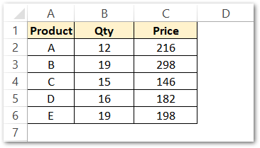
Let us suppose we have the following data in excel:-

In order to check the already existing named ranges in the workbook, press the Ctrl F3 key. This opens the Name Manager Dialog Box.

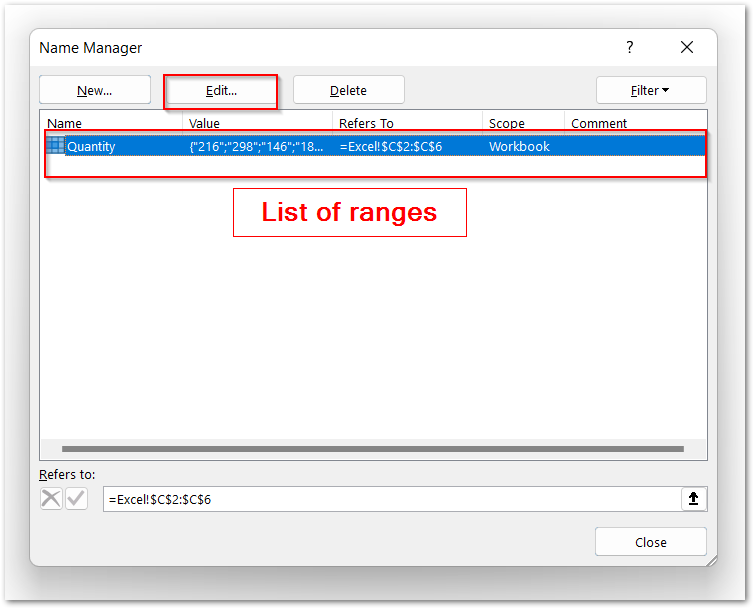
Here you will see the list of named ranges in the entire workbook. Here we got only one named range “Quantity”. Double Click on it on the list or simply select it and then press the Edit button at the top of the list.

As a result, this opens the Edit Name Dialog box. Here you can edit the pre-existing named range “Quantity”.

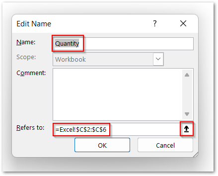
From here, we can change the name and reference of the named range. Here we can see that the “Quantity” is referring to range C2:C6 (“Excel” is the sheet name ) which points to the Price Column.

Click on the Arrow button next to the Refers to Field in the Edit Name dialog box. Select the range B2:B6 on the worksheet.

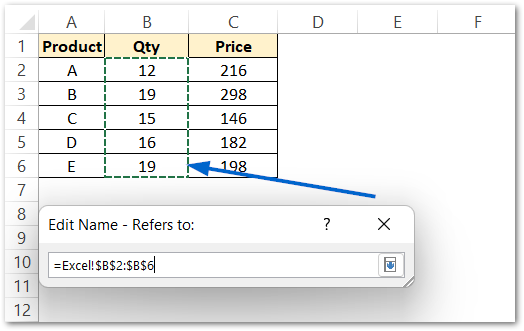
This updates the named range and now the “Quantity” range refers to the range B2:B6.

How to Use Named Ranges in Data Validation?

Data Validation refers to the restrictions imposed on the cell input data. We can use a drop-down list from which we can choose the cell contents. This is known as Data Validation with Drop Down List.

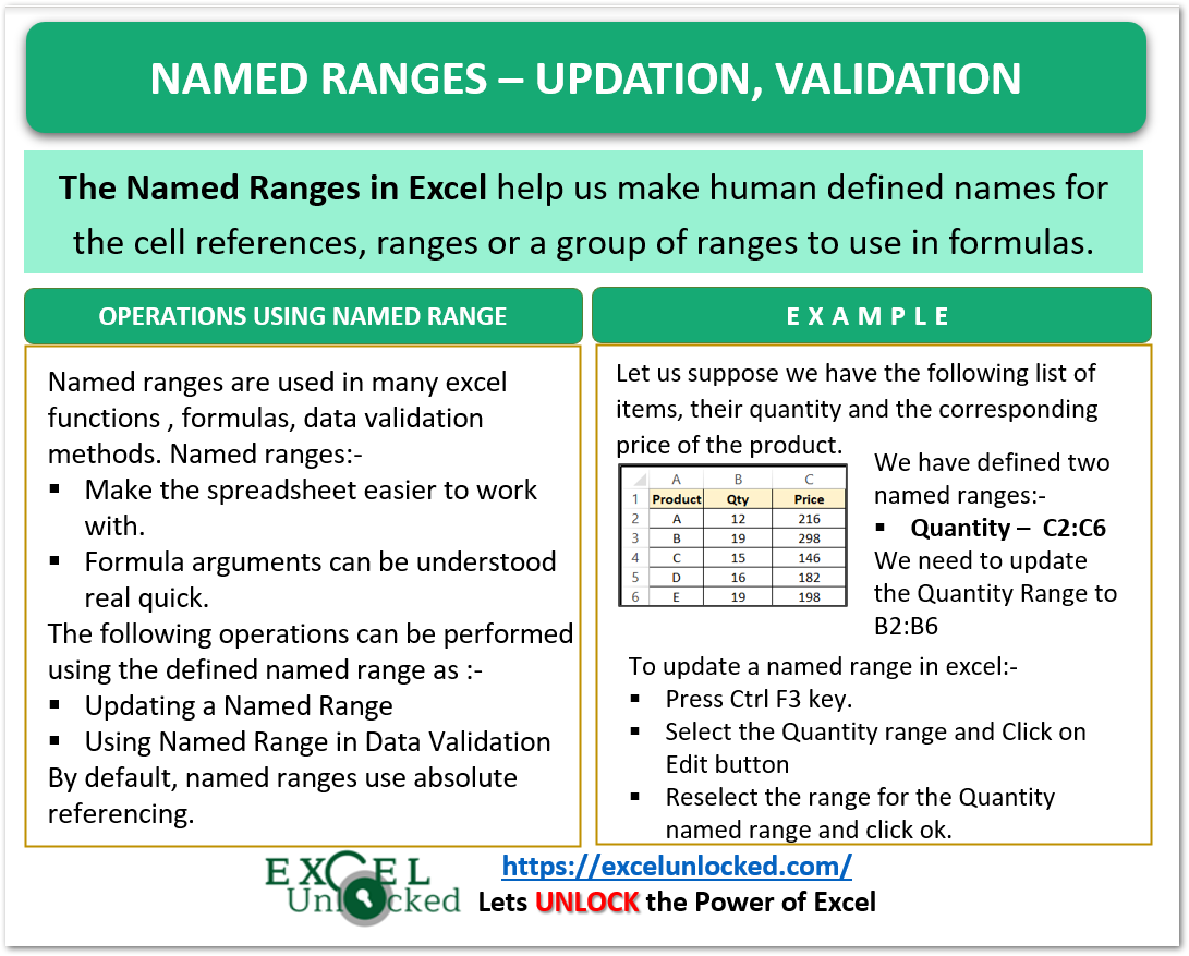
Let us suppose we have the following list of Fruits available in the shop.

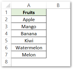
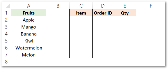
Here we are taking another range in which we want to fill the different orders for the fruits in the shop:-

Creating a Named Range

Either we can manually fill the Item column for the orders or we can make a drop-down list from the range A2:A7.

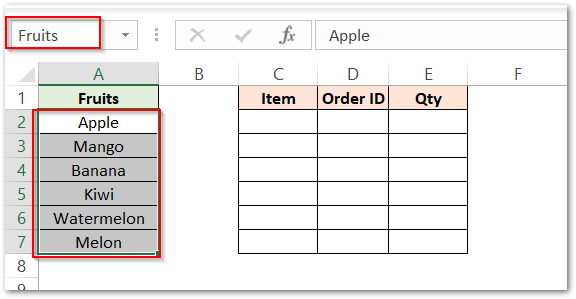
Let’s start by naming the range A2:A7 as fruits:-

• Select the range A2:A7.
• Type “Fruits” in the Name Box.

Using the Named Range as Drop Down List

Now we can use this named range in excel to apply Data Validation on the Item Column. To make a drop-down list, follow the below-mentioned steps:-

• Select the range C2:C7.
• Go to the Data Tab on the ribbon
• Click on the Data Validation button in the Data Tools Group.
• Choose the option List on the Allow field of the Data Validation Dialog Box.

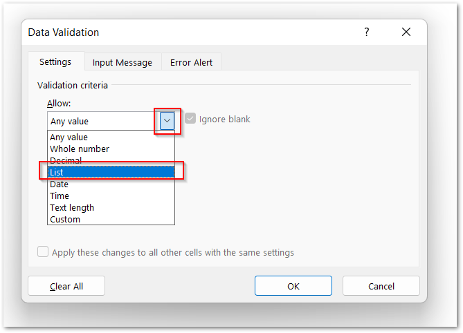
• Type =Fruits in the Source Field.

• Click Ok.

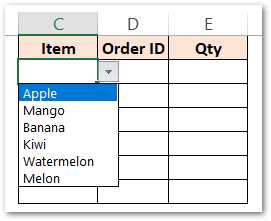
As a result, the Item column of the list has a drop-down list when you start filling the orders.

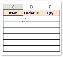
Either click on the Down arrow button next to cell C2 to fill the contents of cell C2 from the drop-down list.

Multiple Ranges, One Named Range

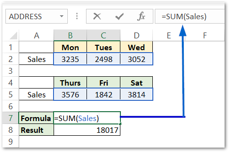
There are times when the data belonging to one category is not contained in the adjacent cells. For Example:-

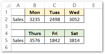
Here the sales are contained in two ranges B2:D2 and B5:D5. To make a named range “Sales” from the two ranges, perform the following steps:-

• Press the Ctrl F3 key. Click on the New button.
• In the Name, type “Sales”.
• Click on the Arrow next to Refers to Field.
• Select the range B2:D2. Press + and then select range B5:D5.

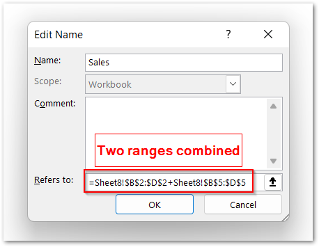
• Click the Ok button.

As a result, the “Sales” points to the sales of six weekdays. Using the Formula:-

=SUM(Sales)

Returns the sum of sales for the entire week.

Consequently, this brings us to the end of the blog.

Thank you for reading.