Sort Data in Pivot Table – Fields, Rows, and Sub Totals

Sorting our data plays a very important role in easily getting the correct order of things, maximum and minimum results and we can even sort the data alphabetically. We have learned to sort the data in tables in excel. In this blog, we will learn how to sort data in the pivot table.

Let us start working! 😎

Taking an Example of Pivot Table for Sorting

We have taken a pivot table having the pizza sales along with taxes, pizza size-wise as well as Category-wise as follows:-

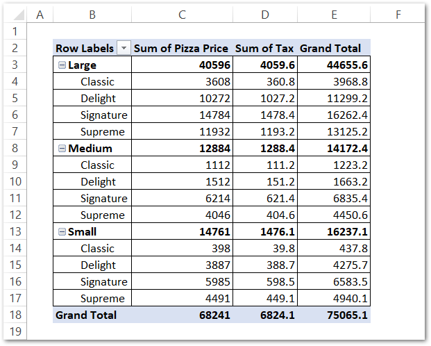
Following are the fields and area sections of this pivot table.

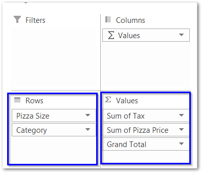
• Rows Section – We have taken the pizza size ( Small, Medium, and Large ) and then we have further divided the pizza size into Pizza Categories (Delight, Classic, Signature, and Supreme ).
• Values Section – In the values, we have three fields Pizza Price, Tax on it, and then the Grand Total ( Pizza Price + Taxes included ). The Grand Total is a Calculated Field.

Sorting the Rows Alphabetically

We would start by sorting the Pizza sizes alphabetically in reverse order ( from Z to A ) All you need to do is:-

Click on the icon and mark the option for Sort ( Z to A )

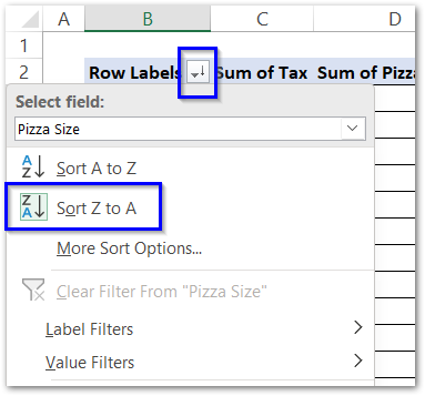
This will sort our pizza sizes from Large, Medium, Small to Small, Medium, Large

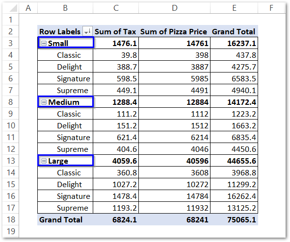
Sorting the Sub Category for Rows

We have divided the Pizza Sizes into Pizza Categories. We can sort them also, but without the use of a button.

To sort the Pizza Categories ( Classix, Delight, Signature, and Supreme ) simply:-

• Right, Click on any one of the Pizza categories in the Pivot Table.
• Click on the Sort option and then choose from Z to A.

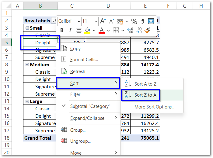
This sorts our Pizza Categories to Supreme, Signature, Delight, and Classis as follows:-

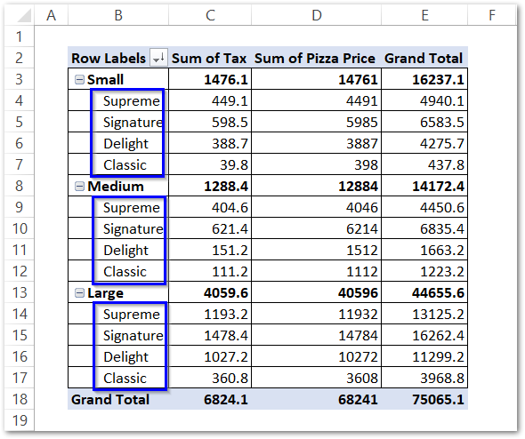
Sort Subtotals in Pivot Table

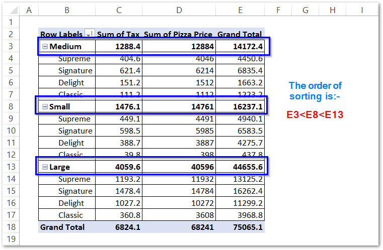
Let us suppose that we want to sort the Pizza Sales (Grand Total = Pizza Price + Tax ) in ascending order Pizza Size-wise ( Small, Medium, and Large). For this:-

• Right-click on cell E3 ( sale of different pizza size-wise ) and choose the sort option from the shortcut menu.
• Select the option for smallest to largest.

Sorting the Values in Descending Order

By now, we have been sorting the rows ( Pizza Size and Pizza Category wise ). In this section of the blog, we will sort the values ( Taxes, Pizza Price, and Grand Total ) in decreasing order. To do this:-

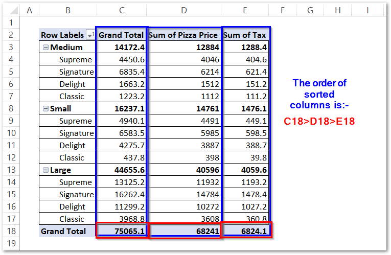
• Right Click on any one of three cells ( C18 or D18 or E18 ) and then choose the sort option.
• Select the option for Sort Largest to Smallest.

This gives us the sorted order of columns on the basis of its grand total.

This is how we sort the items in the pivot table. We can even manually sort the pivot table and there are also some more sort options.

We have come to the end of the blog.

Thank you for reading.