In the previous blog, we learned the Fundamentals of Pivot tables and how to make recommended pivot tables as per our data set. In this article, we will make the pivot tables as per our needs and not what excel recommends by using a blank pivot table.
Nuts and Bolts of a Basic Pivot Table
In order to make a pivot table from scratch, we must learn what components that make a pivot table exist.
- Pivot Cache – The pivot table is the fastest way to flip the way you are looking at your data set. We can change the structure of a pivot table along with the information in seconds. This is so because the copy of actual data is created as a Pivot cache which is very fast, making the pivot table the most efficient tool.
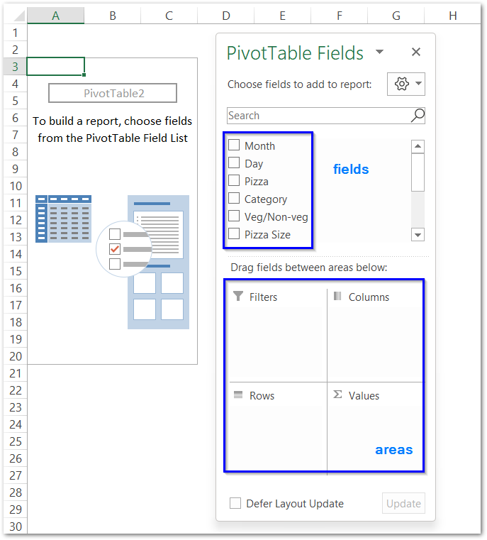
In the above figure, you are looking at a blank pivot table in excel. This is a blank pivot table as it has not picked anything from the pivot cache and thus gives us no insights.
On the left is the Pivot Table Fields pane which contains:-
- Fields – This contains the name of each column from our source data table ( known as fields in pivot tables ). We can drag and drop each of them into the area section which will further decide the pivot table’s structure. An unmarked field means that is not getting used in the pivot table.
- Areas – This area is made of four sections as explained below
- Values – These are the actual values of insights that our pivot table contains. It can be sum, count, average, or percentage.
- Rows – This will contain the fields that become the rows in our pivot tables.
- Columns – This contains the field-making column headings.
- Filters – We can apply filters on our pivot table based on any column value.
However, it is now mandatory to specify all the area sections, not even any of them
Creating a Pivot Table
For instance, let us say we have the sales data of different pizza orders for pizza hut as follows:-
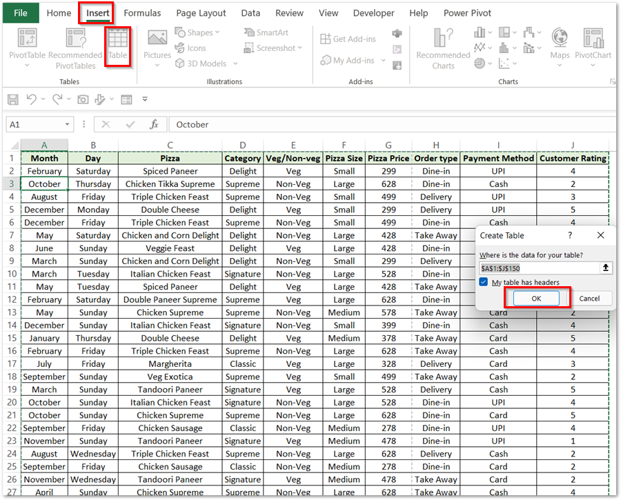
We have created a table from our source data. Select any cell from the table and then:-
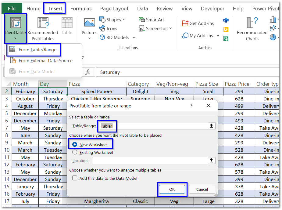
- Go to the Insert tab on the ribbon and click on the Pivot Table button in the Tables Group.
- Click on the option for From Table/Range
- Excel will automatically pick up the table from your currently opened spreadsheet. The default location of the pivot table is a new worksheet.
This will insert a blank pivot table in a new worksheet and the fields section of the Pivot Fields pane would contain the names of columns from our source data table.
- Month – The month in which the order was placed.
- Day – Day of the week.
- Pizza – This is the type of pizza ordered.
- Category – The category of pizza.
- Veg/Non Veg – This tells whether the order was vegetarian or nonvegetarian.
- Pizza Size and Pizza Price
- Order Type – This is the way in which the customer preferred their pizza to them.
- Payment Method and Customer Rating
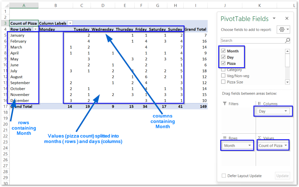
In the above example of a manually created pivot table, we have created a pivot table that tells us the number of pizzas sold on the different days of the week for different months of the year.
We have dragged the following fields into the defined areas:-
- Count Pizza into the Values area.
- Months into Rows Area
- Days into Column Area
Flipping a Pivot Table
Modifying a pivot table simply means that we want to change its field in the area sections. We can replace the Columns with rows and this will flip our pivot table. To change the area section of Month Fields from Rows Area to Columns area:-
- Hover on the Month field in the rows section and a pointer + cursor will appear along with the cursor arrow. Hold the left click on the Month Field in the rows area and drag it to the columns field
- Hold the left click on the Days Field in the rows area and drag it to the rows field.
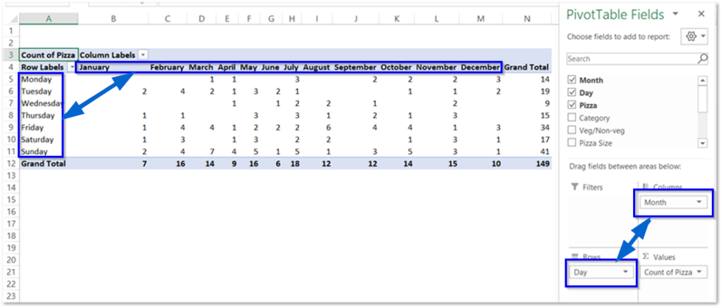
As a result, we have flipped our pivot table successfully.
To delete a field from the area section –
- Unmark the field from the fields section
- Or you can drag and drop that field out from the areas section.
Consequently, this brings us to the end of the blog.
Thank you for reading,

