You are in the third tutorial of the Free ExcelUnlocked Pivot Table Course in Excel. In our previous tutorials, we have gone through the overview and basics of Excel pivot tables and how to create and use a pivot table in Excel. In this tutorial, we would unlock the Pivot Table Grand Total and Subtotal.
What You Would Learn Here
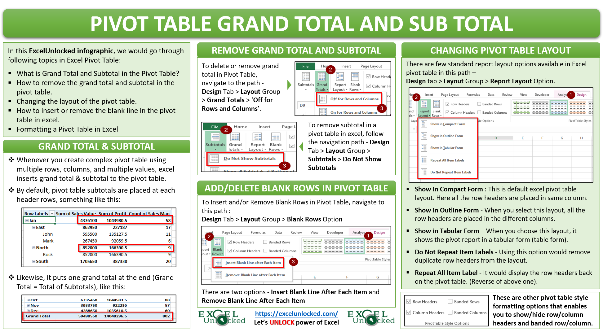
- What is Grand Total and Subtotal in the Pivot Table?
- How to remove the grand total and subtotal in the pivot table.
- Changing the layout of the pivot table.
- How to insert or remove the blank line in the pivot table in excel.
- Formatting a Pivot Table
Before you start moving further with this tutorial, click on the ‘Download‘ button below to download the sample file for practice.
I have created one sample pivot table which I would be using through out this blog.

Create a similar drag and drop pivot table using the downloaded sample data file and practice along.
Excel Grand Total and Subtotal in Pivot Table
Whenever you create a complex pivot table using multiple rows, columns, and multiple values, excel inserts grand total and subtotal to the pivot table.
By default, when you create a pivot table in excel, it puts the subtotal at each header row. For example, in our sample data image (above), there are three rows in the pivot table (Months, Zone and Sales Man). Therefore, excel has inserted subtotal at each of the three levels (rows) and one grand total at the end.

Similarly, a grand total is placed at the end of the pivot table as shown in the image below:

The Grand Total and Subtotal options formatting options are available in the ‘Design’ Tab. Simply, click anywhere on the pivot table and as a result, new tabs would add to the ribbon named – ‘Analyze‘ and ‘Design‘.
Click on the ‘Design‘ Tab and under ‘Layout‘ Group, you can find two options – Subtotals and Grand Totals, as shown below.

Removing Grand Total and Subtotal in Pivot Table
To delete or remove grand total in Pivot Table, navigate to the path – Design Tab > Layout Group > Grand Totals.
From the list of drop-down options, select the option that says – ‘Off for Rows and Columns‘, shown below.

This would instantly remove the grand totals (both rows and column) from the excel pivot table.
To show the pivot table grand totals back, select the option that says – ‘On for Rows and Columns‘ from the drop-down options.
To remove or delete subtotal in a pivot table in excel, follow the navigation path – Design Tab > Layout Group > Subtotals.
From the list of drop-down options, select the option that says – ‘Do Not Show Subtotals‘, as shown below:

This would instantly delete the subtotals at all the levels (row headers) from the pivot and the resultant report would look like this –

Changing the Layout of the Pivot Table in Excel
There are a few standard report layout options available which you can use to change the look of the pivot table. These are available here – Design tab > Layout Group > Report Layout Option.

These are quite self-explanatory.
- Show in Compact Form – Whenever you create any new pivot table report in excel, the excel displays it in the ‘Compact’ form, meaning it is the default layout. Here all the row headers (in our case Month, Zone, and Sales Man) are placed in the same column.

- Show in Outline Form – When you select this layout, all the row headers (i.e. Month, Zone, and Sales Man) are placed in the different columns, like this –

- Show in Tabular Form – As the name in itself says, it shows the pivot report in a tabular form. By looking at the pivot report in the outline form and the tabular form, you would not find any difference. But, if you check both of those minutely, the difference is clearly visible. Our pivot table in tabular form would look like this –

- Do Not Repeat Item Labels – Using this option would remove the duplicate row headers from the layout. The pivot table here would look much cleaner. This option is applicable only when your report is formatted as Outline or Tabular Form, and not in any other layout.

- Repeat All Item Label – This option performs exactly the reverse of the above one. It would display the row headers back on the pivot table.

How to Add or Delete Blank Rows in Pivot Table
By default, all the items (row headers) are stick to each other in a way that there are no blank spaces between two-row headers. It looks a bit difficult to read to the pivot table. However, you can insert a blank row after each row headers (item) by using the following path:
Design Tab > Layout Group > Blank Rows Option > Insert Blank Line After Each Item, as shown below:

As soon as you click on this option, the result would be like this:

If you wish to delete the blank rows in Pivot Table, then use the same path – Design Tab > Layout Group > Blank Rows Option > Remove Blank Line After Each Item.
Other Formatting Options in Pivot Table in Excel
There are other Pivot Table Style formatting options available that you can use to format the pivot table in Excel.
Design Tab > Layout Group > PivotTable Style Options

Use these checkboxes to format your pivot table. For example, the checkboxes ‘Row Headers‘ and ‘Column Headers‘ when unticked, would hide the respective headers from the pivot table.
The options ‘Banded Rows‘ and ‘Banded Columns‘ would highlight the alternate rows or columns (as the case may be).

Congratulations !!
With this, you have completed the third milestone of the excel pivot table course by ExcelUnlocked. Check out the next tutorial on Group and Ungroup Data in Pivot Table.
Check out other Excel Pivot table related blogs on Free Pivot Table Course by Excelunlocked.