In this fourth tutorial of the Free ExcelUnlocked Pivot table course, we would unlock the technique to group dates in the pivot table by years, months, days, hours, minutes, and seconds in Excel. We would also learn how to group the dates by weeks in the excel pivot table.
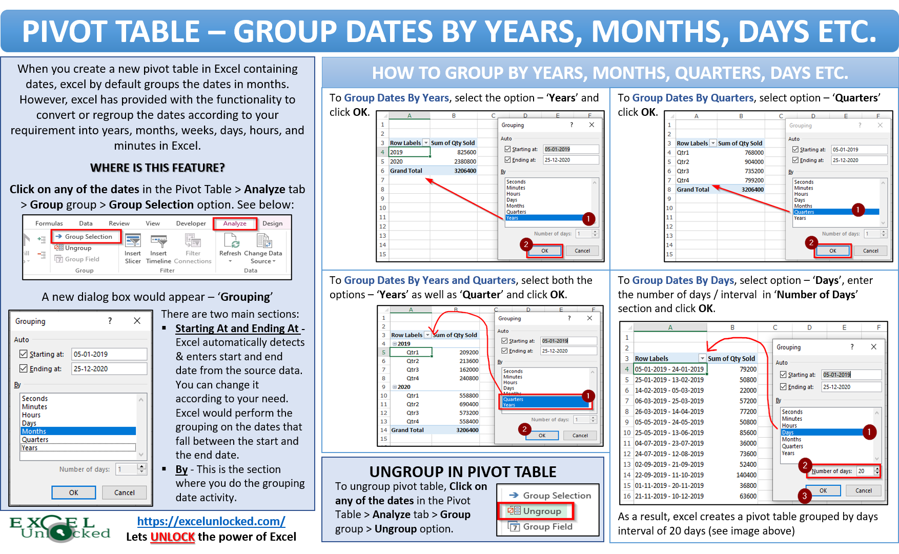
When you create a new pivot table in Excel containing dates, excel by default groups the dates in months. However, excel has provided functionality to convert or regroup the dates according to your requirement into years, months, weeks, days, hours, and minutes in Excel.
Before, you start learning this feature, download the sample file. Click on the download button below and practice as you read.
Navigation To This Feature
To navigate to the group dates feature, follow this path –
Click on any of the dates in the Pivot Table > Analyze tab > Group group > Group Selection option (as shown below).
Also Read: Pivot Table – Group Numbers and Create Range

As soon as you click on the ‘Group Selection’ option, a dialog box would appear named – ‘Grouping‘.
There are two major sections in this dialog box:
- Starting At and Ending At – Over here, Excel automatically detects and enters the start and the end date from the source data. However, you can change it according to your need. Excel would perform the grouping on the dates that fall between the start and the end date.
- By – This is the section where you actually do the grouping date activity.
Group Dates in Pivot Table Excel
Grouping Dates By Years in Excel Pivot Table
By default, the excel groups the dates by months in Pivot Table. To group it by years, simply follow undermentioned steps:
- Open the ‘Grouping‘ dialog box by clicking anywhere on the pivot table dates > Analyze tab > Group group > Group Selection.
- In this dialog box, by default, the option ‘Month’ would be selected. Click the ‘Month’ again to deselect it and then click on the option ‘Years‘ to select it. Finally, click OK to activate the grouping.
As a result, excel would perform summarization of the dates based on years and the resultant pivot table would look like this-

Grouping Dates By Quarters in Excel Pivot Table
To convert the pivot table and group the dates by quarters, follow the undermentioned steps:
- Open the ‘Grouping‘ dialog box by clicking anywhere on the pivot table dates > Analyze tab > Group group > Group Selection.
- Over here, deselect all the existing selected options (by clicking on individual options). Then, click on the option ‘Quarters‘ to select it. Finally, say OK to activate the grouping by quarters in the pivot table.
The result of this would be that excel would summarize the pivot table by quarters.


Grouping Dates By Years and Quarters in Excel Pivot Table
To group the dates by years and quarters, follow the undermentioned steps:
- Open the ‘Grouping‘ dialog box by clicking anywhere on the pivot table dates > Analyze tab > Group group > Group Selection.
- Over here, deselect all the existing selected options (by clicking on individual options). Then, click on the option ‘Years‘ and ‘Quarters‘ to select them. Finally, say OK to activate the grouping by quarters in the pivot table.
As a result, excel would have years first and within the years, it would have quarter wise data, as shown below:

Grouping Dates by Days in Pivot Table Excel
The special thing about the grouping by days in the excel pivot table is that you can specify the number of days or interval by which you want to group your dates.
Like, you can group the dates by 7 days (week) or by 15 days interval, or by an interval of 20 days and like wise.
To achieve this, follow the undermentioned steps:
- Open the ‘Grouping‘ dialog box by clicking anywhere on the pivot table dates > Analyze tab > Group group > Group Selection.
- Over here, deselect all the existing selected options (by clicking on individual options). Then, click on the option ‘Days‘ to select it.
- As you can you click on the ‘Days’ option, the ‘Number of Days‘ would get activated. Type the number of days interval over there and say OK. For weeks, specify 7 days and likewise.
As a result, your pivot table would look like this –

A limitation of grouping by days is that excel will not allow you to group in any other way (like year/month) when you group the dates by days.
In a similar manner, you can group the dates by hours, minutes, and seconds (individually or in combination) using the other options.

How to Ungroup in Pivot Table Excel?
To ungroup the pivot table dates, the path is simple.
Click on any of the dates in the Pivot Table > Analyze tab > Group group > Ungroup option.

With this you have completed the fourth milestone of the ExcelUnlocked Pivot Table course.
Check out other Excel Pivot table related blogs on Free Pivot Table Course by Excelunlocked.