Multiple Ways to Hide Zero Value in Excel

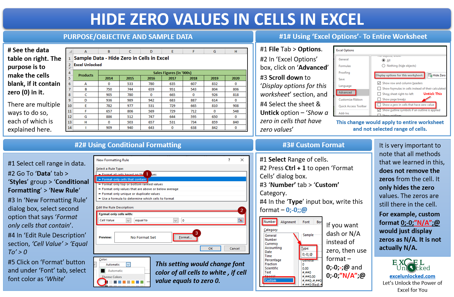
Many a time, you may want to hide the zero value in a cell in Excel. In this blog, we would unlock the technique to make the cell as blank, if you enter zero 0 in a cell in Excel.

As we go through this blog, we would learn multiple ways to show or hide zeros in cells in excel.

Before going through each of these ways, let us first make our sample data ready for use.

Sample Data – Hide Zero Values in Cell in Excel

As you can see from the above image, there are many cells that contain zero value. The purpose now is to hide zero in the cell and make the cell blank.

Download the sample file using the ‘Download‘ button below and practice as you read.

Ways to Hide Zero Value in Cell in Excel

Below are ways using which you can make the cell value as blank, if it contains zero value.

• Automatically Hide Zero Value Using File Options
• Hide Zero Value Using Custom Number Formatting
• Hide Zero Value Using Conditional Formatting
• Write Dash Instead of Zero
• Write ‘Not Applicable’ Instead of Zero

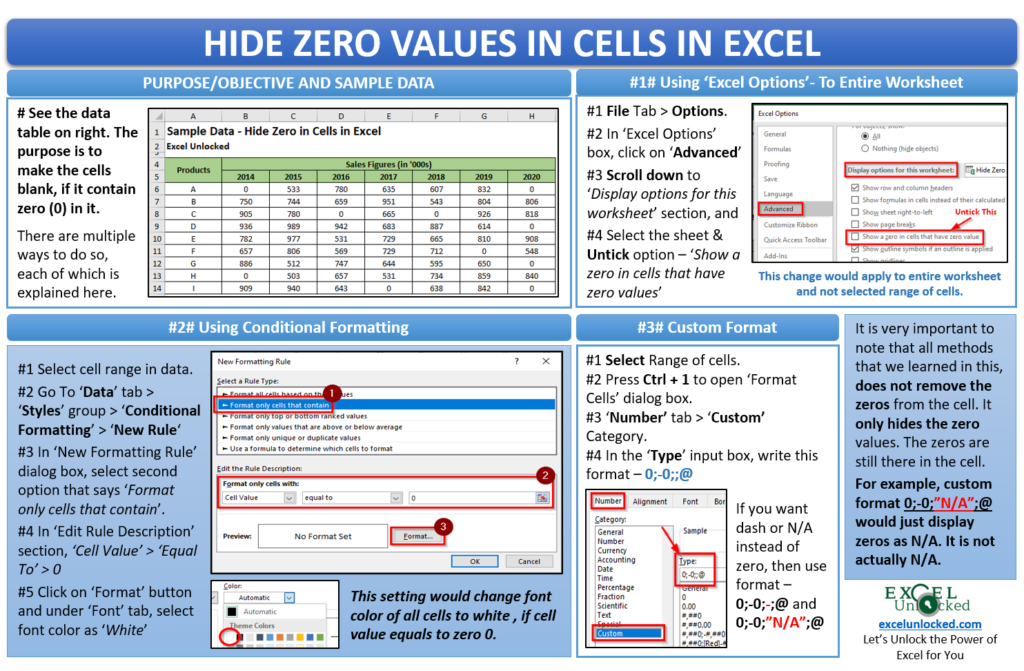
Before getting into each of these methods in detail, it is important to understand the impact of the above methods. Hiding Zero in Excel using any of the above methods does not mean that it has completely removed zero. The zero still remains in the cell, but it is simply hidden and is not visible.

Automatically Hide Zero Value Using Excel Options

This is the simplest, fastest, and quickest method to hide zero in cells in Excel using Excel inbuilt functionality. However, it is important to note that this change applies to the entire worksheet, and not to selected cells or range of cells.

Follow the undermentioned steps-

Navigate to the following path in Excel workbook – File Tab > Options Button. The ‘Excel Options‘ dialog box Would appear on your screen. Click on the Advanced button, and use the scroll bar to search for the “Display options for this worksheet” section.

Here, untick the checkbox that says ‘Show zero in cells that have zero values‘ (This checkbox is tick by default) and finally, click on ‘OK’. Below image is self-explanatory.

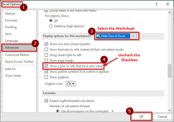
As a result of this change, all the zeros in the worksheet would get hidden immediately. Note that, zeros are not removed, but the cells still contain zero 0.

This method, as mentioned earlier, would apply to the entire worksheet. To apply it only for a selected cell range, use other methods.

Hide Zero Value Using Custom Number Formatting

The Custom Number Formatting is a number formatting feature provided by Excel that allows us to create our own format for numbers (positive, negatives and zeros) as well as texts. It also allows us to create our own custom format for date/time.

We can use this custom number formatting feature to hide the zero in cell. Follow the below steps:

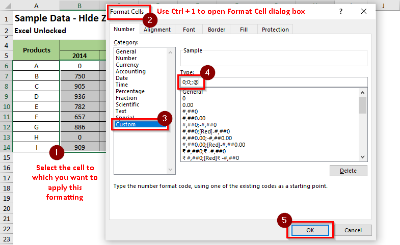
As a result, you would notice that excel converts zero into blank.

Hide Zero Value Using Conditional Formatting

Another way to hide the zero values in all the cells in excel is by changing the font color of the cell if it contains 0. This can be achieved using the conditional formatting feature in Excel.

Follow the below steps to achieve the same:

Select the cell range that contains the values (i.e. B6:H14). Now, navigate to Home Tab > Styles Group > Conditional Formatting option > New Rule Option.

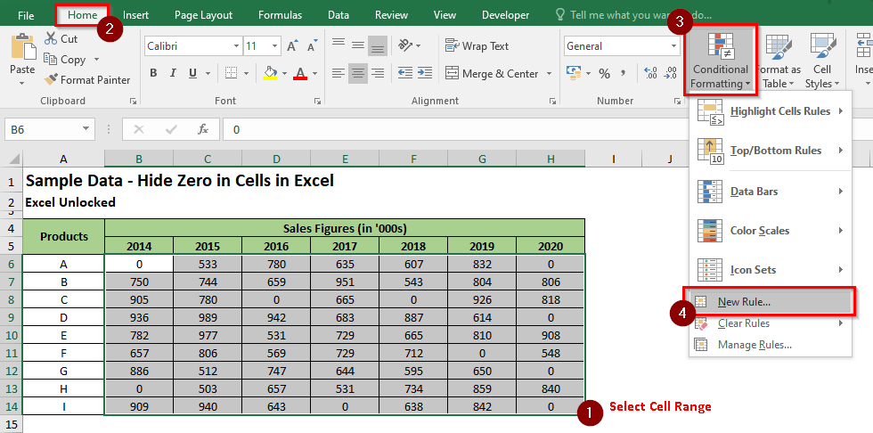
The ‘New Formatting Rule’ dialog box would appear on your screen. In it, select the second option – ‘Format Only Cells that Contains’ and make settings and click on the ‘Format’ button.

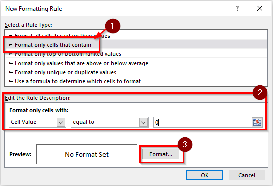
Select the Font Color as White and click OK to all the dialog box.

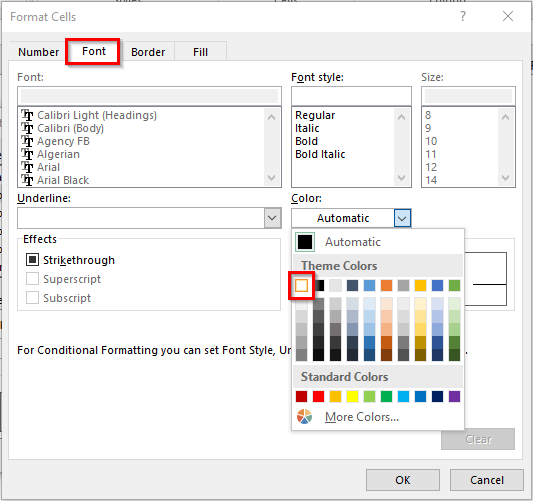
As a result, all the cells that has zero in it will have font color as white and hence not visible in the cell (because of white cell background).

Write Dash Instead of Zero

There are two ways to convert zeros into the dash symbol. The first one is the ‘Accounting‘ number formatting and the other one is the ‘Custom‘ number formatting.

The ‘Accounting’ number formatting is also one of the cell formatting options which are used to format the amounts in excel.

Using ‘Accounting’ Format to Insert Dash

Select the range of cells to which you wish to apply the formatting, and use any of the below mentioned path-

Go to ‘Insert‘ tab > ‘Number‘ group > ‘Comma Style‘ option/button.

Press Ctrl + 1 to open the ‘Format Cells’ dialog box and select the category as ‘Accounting‘ and click on ‘OK’, as shown in the image below

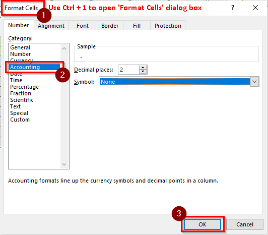
Using Accounting Number formatting would convert all the zeros into dash in the selected excel cell as shown in the image below:

Using ‘Custom’ Format to Insert Dash

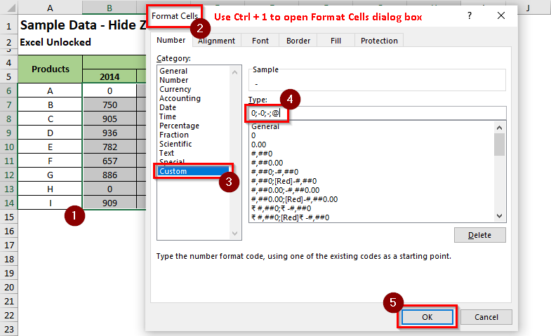
Similar to the ‘Accounting’ number formatting, we can also use the custom number formatting to insert dash. This can be achieved by simply writing dash (-) in the third section of the custom number format, like this: 0;-0;-;@

Select the range of cells and use keyboard shortcut Ctrl + 1 to open the ‘Format Cells’ dialog box. From the list of categories, select ‘Custom’ and enter the format 0;-0;-;@ in the ‘Type’ input box. Finally, click on the ‘OK’ button as shown in the image below

Write ‘Not Applicable’ Instead of Zero

Now, when you are a bit familiar with the custom number formatting in Excel, writing the text ‘Not Applicable’ instead of zero is not a challenging task.

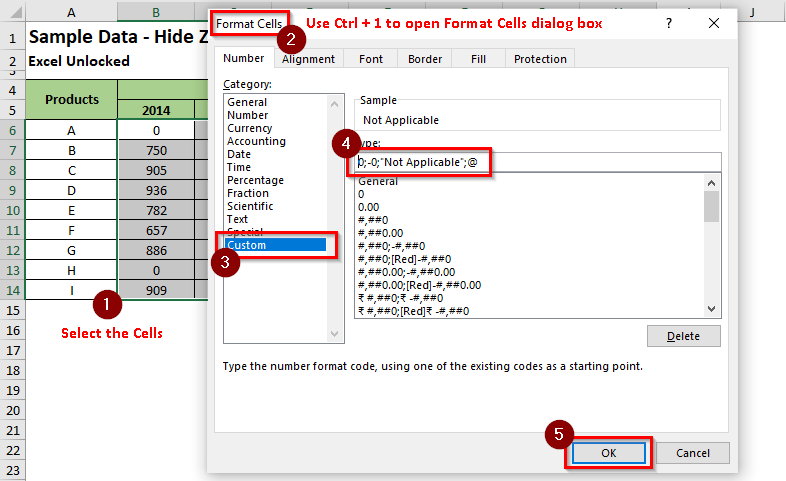
Select the range of cells and use keyboard shortcut Ctrl + 1 to open the ‘Format Cells’ dialog box. From the list of categories, select ‘Custom’ and enter the format 0;-0;”Not Applicable”;@ in the ‘Type’ input box.

The result would be as below:

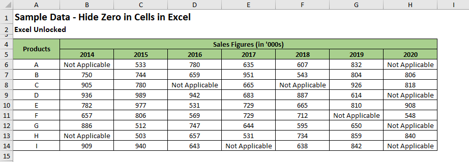
Note that only formatting of the cell has been changed, and not the cell value. Cell still contains the value zero, but it displays the word “Not Applicable”.

With this, we have reached the end of this blog. Share your views and comments in the section below.