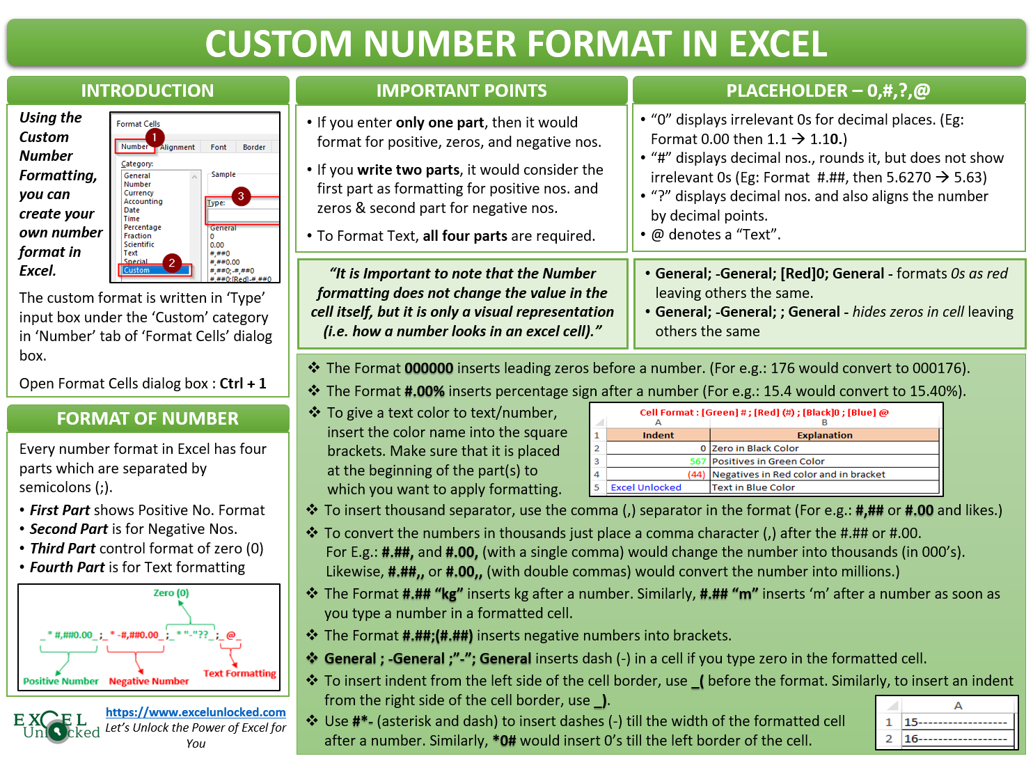
While working with cells in Microsoft Excel, you may have come across various pre-defined cell formats that you can use to format the numbers, etc. But, many a time, you may have a requirement to have something different than what the excel has provided. With the custom excel number format option in Excel, you can create your own custom format that meets your needs.
The custom excel number format is a very powerful tool that may seem to be complex, but trust me, it is very easy if you understand its structure.
- Where is the Custom Excel Number Format Feature?
- Unlocking Custom Excel Number Format Symbols
- Some Important Points To Note
- Four Basic Placeholders
- Insert Zeros Before A Number in Excel
- Insert Percentage % Using Custom Excel Number Format
- Using Colors in the Custom Formatting
- How to Insert a Thousand Separator ?
- Using Custom Format to Change Numbers into Thousand
- Enter Text and Numbers in The Same Cell
- Special Symbols in Custom Number Format
- Currencies in Custom Number Format
- Convert Number to Fraction in Excel
- Show Negative Number in Bracket
- Show cells containing Zero as Blank or Dash
- Adding Indents in Custom Excel Number Format
- Repeat Character in Cell Till Column Width
- Custom Formatting If Condition Fulfils
In this tutorial, we would unlock this feature in Excel and master you with the excel number format.
Where is the Custom Excel Number Format Feature?
The Excel Custom Number Formatting feature is available in the ‘Format Cells’ dialog box under the ‘Numbers’ tab.
You can use any of the below paths to navigate to the ‘Format Cells’ dialog box.
- Right-Click on the Cell to Format > Click ‘Format Cells’ option
- Home tab > Number group > Drop-Down button > More Number Format button
- Home tab > Number group > Format Cells dialog box launcher
- Keyboard shortcut – Ctrl + 1 or Alt + H + FM
In the Format Cells dialog box, under the ‘Numbers’ tab, you would find the ‘Custom’ category. Click on this category and you would find the ‘Type’ input box. In this input box, you can enter your own customized format. It would get saved for future use, once you click on the ‘OK’ button.
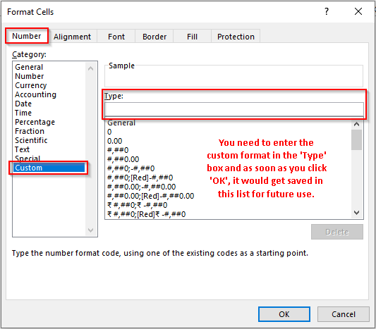
Instead of creating a new format from scratch, you can use the pre-provided custom number format from the list (as you can see from the screenshot above). However, in order to use these weird-looking formats, you need to first learn what these symbols mean.
Also Read: Format Cell Content – Excel ‘Number’ Format
Unlocking Custom Excel Number Format Symbols
In order to learn to create your own new format, it is important to first know how Excel read and understand these symbols.
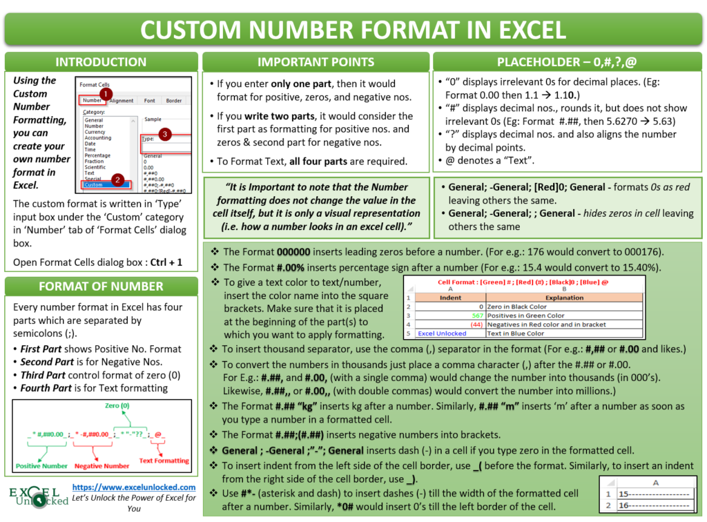
Every number format in Excel has four parts which are separated by semicolons (;).
- First Part – It denotes the formatting for a positive number
- Second Part – It represents the negative number formatting
- Third Part – It denotes formatting for 0 (zero)
- Fourth Part – It represents formatting for a text
Let us take one pre-defined number format to understand it and summarize in a pictorial manner.

However, it is not mandatory to write a custom format like above (with semicolon separators) for all the four parts. Below is the way excel reads the custom format when you do not use all the four parts:
- If you enter only one part, then excel would consider it as a format for all the numbers (positive, zeros, and negative numbers).
- If you write two parts, then excel would consider the first part as formatting for positive numbers and zero and the second part for negative numbers.
- Excel would only read the formatting for a text if all the four parts are written in the ‘Type’ input box.
Some Important Points To Note
It is pertinent to note that the Number formatting does not change the value in the cell itself, but it is only a visual representation (i.e. how a number looks in an excel cell).
If you want to apply the default format for all the parts except any of the middle part, then type the word ‘General’ for those to which you want to apply the default excel format. For Example:
Also Read: Change And Convert Number To Text in Excel
General; -General; [Red]0; General
This would format the positive, negative, and texts as a default excel format, but zero would be in Red color.
If you want to hide any particular type of cell content, then leave that part as blank. For Example, to hide all zeros, the format would be:
General; -General; ; General
There is nothing between the last and the second last semicolons.
Four Basic Placeholders
The four basic placeholders in a custom number formatting, that everyone should know are 0, #, ?, and @.The “0” placeholder displays zeros for the decimal places. For example – If positive number format is #.00, then if you type 1.1 in the formatted cell, the excel would convert it to 1.10.
- The “#” denotes decimal place formatting, but it does not display irrelevant zeros and also helps in rounding the numbers. For example – If the cell is formatted as #.##, then 1.1 will be represented as 1.1 only, but 5.6679 would be displayed as 5.67 (rounded up to 2 digits).
- Similarly, the number 5.6679 with cell formatting as #.### will be displayed as 5.668 (rounded up to 3 digits).
- The “?” placeholder removes unnecessary zeros before and after the decimal places and it also aligns the number in a column by decimal places. For example, #.???? will show a maximum of four decimal places and also align them in a column
- The only text placeholder is “@” which denotes that the formatting should be applied to a text.
However, it is important to note that all the digits in number before a decimal point, will be displayed even if the formatting is set as #.##.
Example – The number 102.44587 in a cell with formatting as #.## will result in 102.45 (all numbers before the decimal point, but only two decimal places after the decimal point.
Similarly, there are many such characters like _(underscore), *(asterisk), “ “(double inverted commas), ,(Commas), /(forward slash), \(backslash), which we would discuss in the latter part of this blog, as we proceed.
Insert Zeros Before A Number in Excel
Many a time, you may want to add leading zeros before a number in Excel, like 000176, to make the number of specific character length (like 6 characters long). But when you type 000176 in an excel cell (having general/number formatting), it would return the value as 176 (because mathematically, the number 000176 is equal to 176).
However, there are multiple ways to insert 0 before a number in Excel. In this section, we would focus on using the custom number format to achieve this task.
Use the format – 000000
Here, the number of zeros should be equal to the number of digits that you want your number to have.
So, when you type 1 in the cell having this custom formatting (000000), it would return the value as 000001. Similarly, 15 would return the value as 000015.
Insert Percentage % Using Custom Excel Number Format
There is a specific category under the ‘Format Cells’ dialog box to insert the percentage symbol to a number in Excel.
Additionally, you can even use custom formatting to insert the percentage after a number in Excel. Use the format – #.00% OR #.##%
Using Colors in the Custom Formatting
You can give different colors to different parts of a custom format. There are mainly eight colors which are supported by the custom excel number format which are:
[Red], [Green], [Cyan], [White], [Blue], [Yellow], [Magenta] and [Black].
Always remember that the color should be written at the starting of the part to which you want to add color formatting. Also, the color names should be included within the square brackets.
Below is an example for your reference:
[Green] # ; [Red] (#) ; [Black]0 ; [Blue] @
This means a positive number would be displayed in green color. The negatives in red color and in brackets. Zero would be displayed as a black colored black and every text would be in blue color.

How to Insert a Thousand Separator ?
To insert a thousand separator, use the comma character (,) followed by digit placeholders (0, # and ?).
For example, #,## or #.00 or any such combination. It is important to note that excel would only insert a thousand separators if the comma is followed by any digit placeholder. For example, #, will not insert any thousand separators, as nothing follows the comma.
The below image shows how the combinations would work.

Using Custom Format to Change Numbers into Thousand
To convert the numbers in thousands just place a comma character (,) after the #.## or #.00 or any such number custom format. Similarly, to convert the numbers into millions, place two commas (,) after #.## or #.00 etc. To round more, keep on adding commas, as required.
Make sure that you do not enter any digit placeholder after this comma(s).
#.##, and #.00, (with a single comma) would change the number into thousands (in 000’s). Likewise, #.##,, or #.00,, (with double commas) would convert the number into millions.
The below image is self-explanatory.

Enter Text and Numbers in The Same Cell
When you simply enter any number followed or preceded by a text character in the same cell, the number loses its number property. It means that excel will not allow you to do any number operation like addition, subtraction, division, and multiplication with this string.
However, using the excel custom number format feature, you can create your own format, without changing the property of a number. Below is the trick.
Just insert the text characters into the double inverted commas (“ “). For example, if you want to write 15.45 kg, then enter #.## “kg” in the ‘Type’ input box.
Similarly, you can combine this trick with the ‘Convert number into a thousand’ trick to show that the numbers are in thousands/millions.
Refer to the below screenshot:
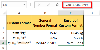
As you can see in the highlighted part in the above screenshot – the number remains a number and did not change its property.
Alternatively, if you wish to enter only one character text after the number then you can even use backslash instead of “ “, – #.## /m
Special Symbols in Custom Number Format
You can even include the special symbols in the custom number format by using the ASCII code for it. Press Alt and then insert the ASCII Code. Below are the ASCII Codes for the respective special symbols:
- TradeMark ™ : Alt+0153
- Copyright © : Alt+0169
- Degree (°) : Alt+0176
- Plus-Minus Sign (±) : Alt+0177
- Micro Sign (µ) : Alt+0181
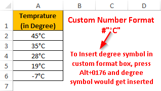
Similarly, you can insert the other special symbols using the ASCII Code.
Currencies in Custom Number Format
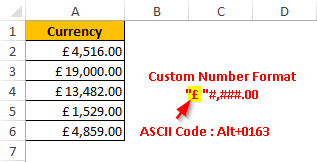
Like the Special Symbols, you can even insert currencies symbols using the Alt key followed by an ASCII code. Below are some of the examples of the ASCII codes corresponding to the currency symbols:
- Euro (€) : Alt+0128
- British Pound (£) : Alt+0163
- Japanese Yen (¥) : Alt+0169
- Cent Sign (¢) : Alt+0162
Convert Number to Fraction in Excel
When your cell(s) format is ‘General’ or ‘Number’, you cannot enter a fraction (numerator/denominator) in that cell. For example, in a ‘Number’ formatted cell, you can write 0.90 but cannot write its fraction form 9/10.
To insert a fraction for a number, excel has pre-provided a ‘Fraction’ category, which we have discussed in one of our previous blogs on ‘Format Cell Content – Excel Number Format’.
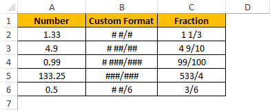
Additionally, you can create your own custom fraction format by writing the format in the ‘Custom’ category.
- Show the proper fraction for a number with the remainder up to one digit – # #/#
- Show the proper fraction for a number with remainder up to two digits – # ##/##
- # ###/### would show the proper fraction for a number with remainder up to three digits.
- ###/### would show an improper fraction for a number (where Denominator is less than or equal to numerator).
You can even create a fixed base fraction number format by entering the fixed base digit after the forward-slash (/) in the cell custom format.
For example, to have a fixed denominator as 6, the format code would be # #/6.
Show Negative Number in Bracket
As discussed at the inception of this blog, there are four parts of any custom number format separated by semicolons.

Just to recall, if you enter only one part/section in the ‘Custom’ category of this dialog box, then excel would apply this formatting to all the numbers.
So, in order to have separate formatting for a negative number, you need to have at least two parts in your custom format. The first part would denote formatting for a positive number and zero and the second part for a negative number.
Now, to display the negative numbers in the bracket (parenthesis), just insert the format inside Round brackets (parenthesis).
Example : #.##;(#.##)
In the above format, the first part (before semicolon represents a positive number and the second part represents negative numbers, and the Round brackets would display them in brackets.
Show cells containing Zero as Blank or Dash
To show the cell that contains zero as dash, you can use the ‘Accounting’ category under the ‘Format Cells’ dialog box. To learn about all the categories, follow our previous blog on ‘Format Cell Content – Excel Number Format’.
Additionally, you can create a new custom format for achieving this. As we know that the third section represents format for ‘zero (0)’, you can enter the dash (-) under double inverted commas to insert a dash in the cell where you enter zero.
General ; -General ;”-”; General
Similarly, to keep the cell as blank, do not enter anything in the third part, and leave it as it is:
General ; -General ; ; General
Adding Indents in Custom Excel Number Format
Where you write any text in a cell in Excel, it is by default left aligned and stick to the left border of the cell. Similarly, a number is by default right aligned and stick to the right border of the cell.
You can, however, add indents and insert one or more character space from the right/left borders of the cell using the underscore (_).
To insert indent from the left side of the cell border, use _( before the format. Similarly, to insert an indent from the right side of the cell border, use _).
Let us take one format and understand – #_) ; (#) ; ; _(@
The above format would insert negative numbers into brackets (#). It would also give an indent from the right border by one character so that the ones digit in the positive numbers are exactly aligned to the ones digit of the negative number #_). The empty third part means zero should get converted to blank. It would also put one character space from the left of the text. Refer to the below image.

To add more than one character indents, use more than one underscores (like – _(_( OR )_)_ would enter two character spaces from left OR right respectively, and so on).
Repeat Character in Cell Till Column Width
The excel custom formatting feature would prove to be a helpful feature when you wish to repeat a specific character until the column width ends.
For example, you want to type a number in a cell, and the excel inserts leading zeros before it (extended up to the left border of that cell)
To do so, first, enter an asterisk (*) symbol and then type the character that you want to repeat.
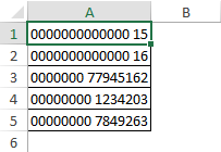
Let’s format our cell-like if you type a number, the excel should lead it with zeros up to the width of the cell. Enter the following in the ‘Type’ input box under the ‘Custom’ category.
*0#
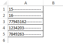
This would insert the 0’s before the number in the formatted cell. The zeros would extend till the width of the cell. Below is the screenshot for your reference.
Similarly, #*- would insert dashes (—–) after the number.
This technique is very useful when you want to change the alignment of the text/number in a cell. By default, every number is right-aligned and a text is left aligned. You can use the below custom format to achieve this.
To Right-align the text, use format: @*
To Left align the number, use format: *#
Custom Formatting If Condition Fulfils
You can use a specific custom formatting if a condition is fulfilled and another formatting if the condition is not fulfilled.
To do so, enter the mathematical operator before the number format enclosed in square brackets [ ].
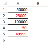
Let’s take one small and simple example. The number should be in red color if the value is less than 50000 and in black color, if it is more than and equal to 50000. Between these two numbers, the color should be black. To achieve this, enter the use the below format:
[Red] [<50000] # ; [Black] [>=50000] #
This brings us to the end of the custom number formatting in Excel.
Share your views and comments in the comment section below.

