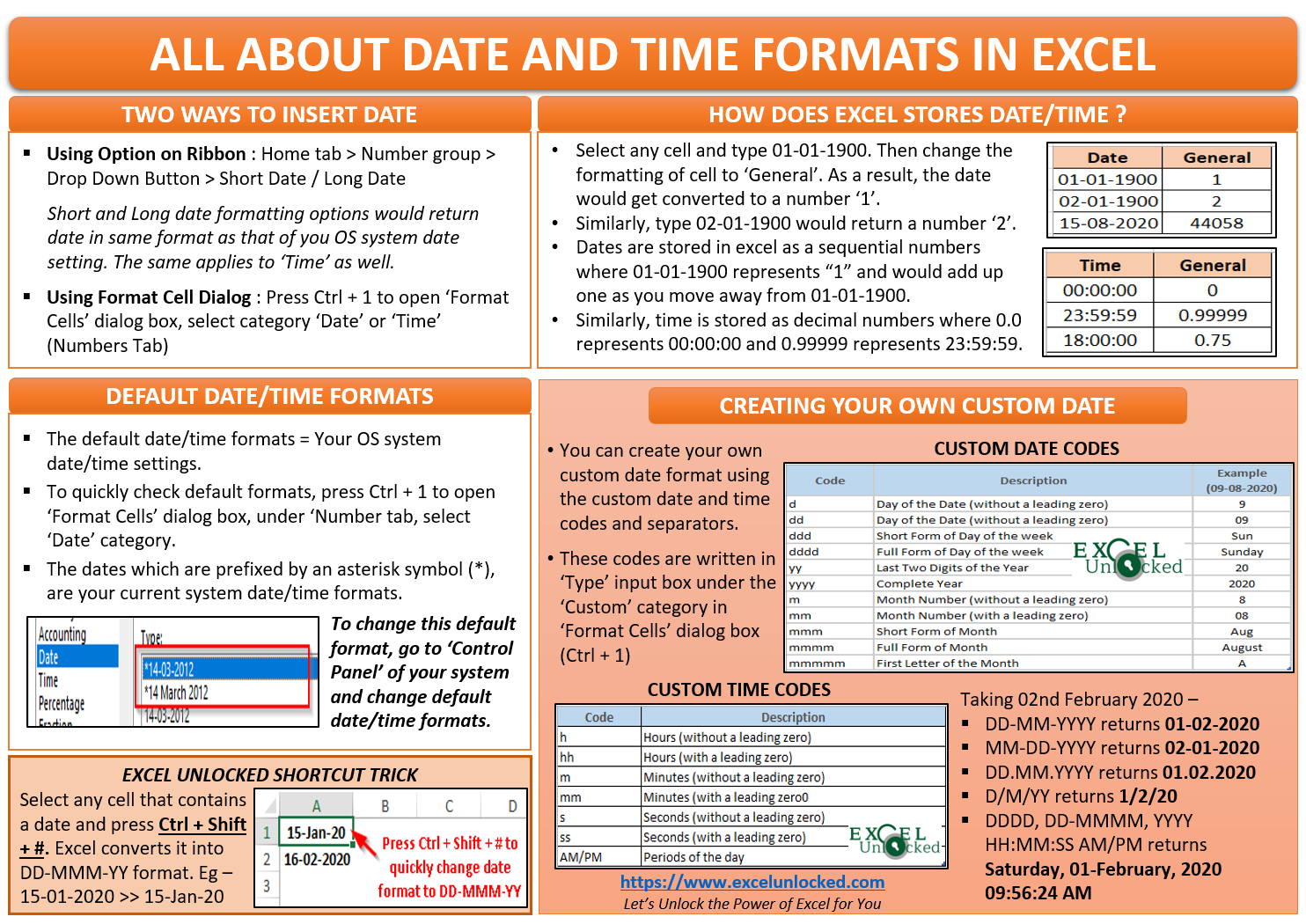
In our previous blogs, we had learned about various types of cell formatting options and the number formatting in Excel. Also, we learned about how to create our own custom number format in Excel. In this blog, we would learn some basics about the excel date format, how does it get stored in backend, what are the default excel date formats and how can we create our own custom excel date format.
How to Insert Date in Excel ?
There are multiple ways using which you can access and insert a date in Excel. Each of these ways would be covered in detail.
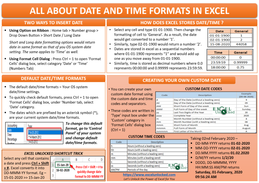
Using Option on Ribbon – This is the most common way that one uses to insert a date in excel. Select the cell to which you want to insert a date, then go to the ‘Home’ tab and click on the drop-down button under the ‘Number’ group as highlighted in the screenshot below.
There are two date options – ‘Short Date’ and ‘Long Date’.
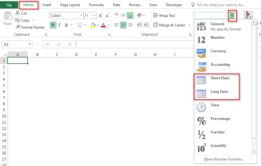
When you select any of these options, the cell format converts into a respective date format. Now, you can easily type the date in the cell and it would work.
Also Read: What is Date and Time Format in Excel?
It is important to note that, the short date and the long date formats would return the same format as the default windows system date formats.
Using ‘Format Cells’ Dialog Box – You can even access various in-built date and time formats by using the ‘Date’ category in the ‘Format Cells’ dialog box. To navigate to it, you can use either of these methods:
‘Home’ tab > ‘Number’ group > Click on the drop-down button > Select the option ‘More Number Formats’
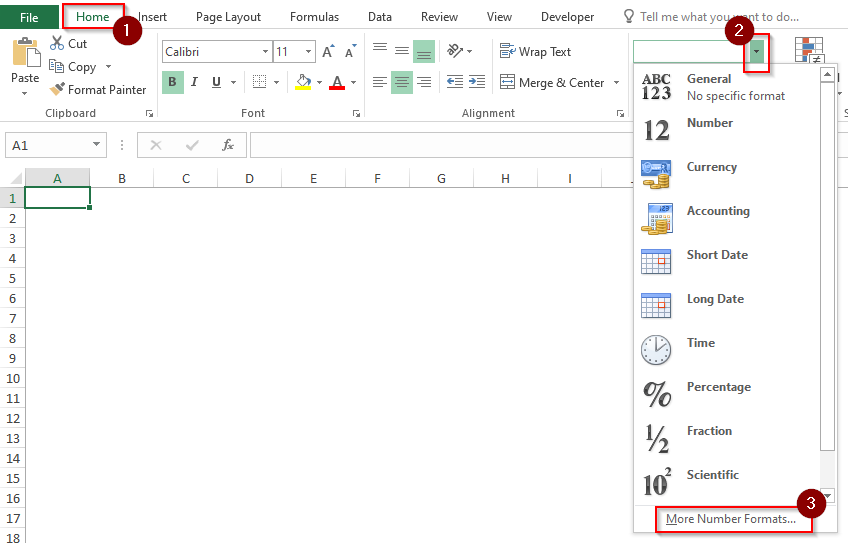
Using Dialog Box Launcher : ‘Home’ tab > ‘Number’ group > ‘Format Cells’ dialog box launcher.

Keyboard Shortcut – Ctrl + 1
All the above options would open the ‘Format Cells’ dialog box. Under the categories section, you can find the ‘Date’ and ‘Time’ categories providing the list of excel in-built date and time formats.
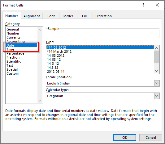
Default Date and Time Format
As mentioned earlier, when you click on the ‘Short Date’ or ‘Long Date’ or ‘Time’ button under the ribbon options, the excel inserts the default windows system date or time format into the cell.
You can quickly check the default date and time format using the Date / Time categories in the ‘Format Cells’ dialog box. Open the ‘Format Cells’ dialog box (using Ctrl + 1), and go to the ‘Date’ category. The first two formats (which are prefixed by an asterisk symbol (*) are the ‘Short Date’ and ‘Long Date’ formats of your windows system.
Also Read: Format Cell Content – Excel ‘Number’ Format
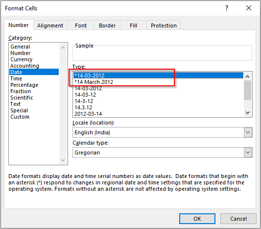
These two would update when you change the default regional date and time formats of your windows system under the control panel.
Changing Default Date and Time
As learned in the previous section, the ‘Short Date’ and ‘Long Date’ formats are nothing but the operating system’s default format. To change this default date and time settings, you need to navigate to the ‘Date and Time’ settings under ‘Control Panel’
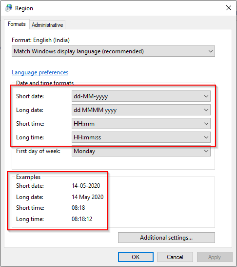
You can change it from here and click ‘OK’. The same would update the default excel date and time formats for a short date and long date.
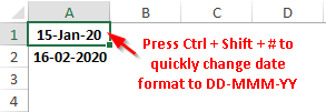
A ShortCut ExcelUnlocked Trick : Select any cell that contains a date and press Ctrl + Shift + #. You would notice that excel converts it into DD-MMM-YY format (Like 15-01-2020 would get converted into 15-Jan-20).
How Excel Reads Date and Time?
This section of this blog would help you to understand how does the excel reads and stores any date or time in Excel.
Every date and time in the Excel cells is stored as a sequential number. The date format like 15-01-2020 in a cell is just a display for you. Behind this date, it is a number which the excel understands.
Let us understand this by taking a small demonstrative example. Select any cell and type the date 01-01-1900 (1st January 1900). Now, change the cell A1 format to ‘General’.
What did you notice? Surprisingly, excel would return the number ‘1’. This means that for excel, the date 01-01-1900 is just a number 1. Similarly, type 02-01-1900 (2nd January 1900) and you would notice that the excel returns the number ‘2’ and so on as you proceed further with the date.
Therefore, if you enter the date as 15-08-2020 and change its format to ‘General’, it would return the number 44058 (which means, that 15-08-2020 is 44058 days after the first date 01-01-1900).
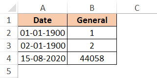
The dates prior to 01-01-1900 are not recognized by Excel.
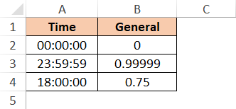
Similarly, the time in excel is stored in excel as decimal numbers. It ranges between 0.0 to 0.99999 where the lowest number represents 00:00:00 (12 AM) and the highest represents 23:59:59.
So, .5 represents 12 PM (12:00:00). Likewise, 0.75 represents 6 PM (18:00:00) and so on.
Consequently, if you enter date and time in the same cell, then it would sum the respective numbers like 15-08-2020 18:00:00 will return 44058.75 and 02-01-1900 23:59:59 will return 2.99999.
How to Find Serial Number of Date in Excel ?
In the previous section, we learned that the excel stores a date and time as a number. But if you want to convert the date to number or time to a number, then one way, as unlocked above, is to change the cell formatting to ‘General’.
However, you can even check the date and time format without changing the cell format by selecting the cells that contain the date/time and then using Ctrl + 1 keyboard shortcut. The ‘Format Cells’ dialog box would appear before you. Under the ‘General’ category, you can see the sample number format of the date/time as highlighted below.
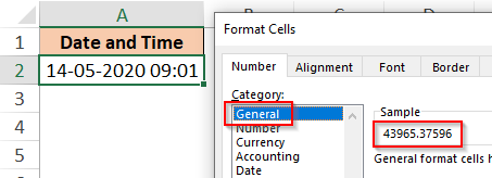
Here, 43965 represents date 14-05-2020, and 0.37596 represents the time 09:01.
You can even use the =DATEVALUE() and =TIMEVALUE() formula to find the date and time serial numbers. These formulas only have one argument viz. Date and time respectively.
Like, =DATEVALUE(“14-05-2020”) would return 43965, and =TIMEVALUE(“09:01”) would return the value 0.37596.
To get both of these in one cell, concatenate the formulas either by using the formula =CONCATENATE(value1,value2) or using an ampersand (&) symbol like value1&value2.
Refer to the below example:
=DATEVALUE(“14-05-2020”)&TIMEVALUE(“09:01”) would return 43965.37596 as the value.
Create Your Own Custom Date
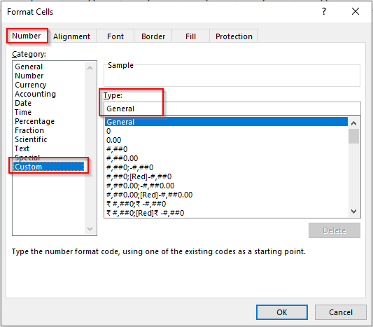
In one of our previous blogs, we learned about how to create a custom number format in Excel. In a similar way, you can create your own custom date and time format in excel in the ‘custom’ category of ‘Format Cells’ dialog box (Ctrl + 1).
The custom format is written in the ‘Type’ input box as highlighted in the screenshot below:
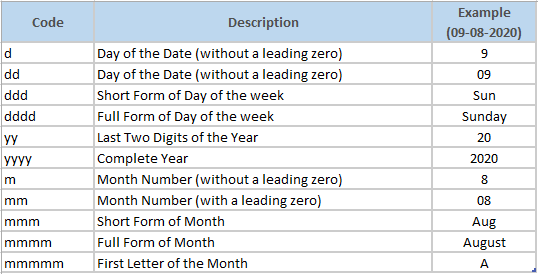
To write a custom date format, you need to first know the custom codes:
Custom Date Codes :
Custom Time Codes :
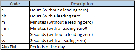
Based on the above codes, you can create custom date and/or time formats as per your need by using any of these separators – dash(-), comma(,), colon (:), slash (/), period(.)
Below are some of the sample formats, but not exhaustive. You can create your own. Taking 02nd February 2020 –
- DD-MM-YYYY returns 01-02-2020
- MM-DD-YYYY returns 02-01-2020
- DD.MM.YYYY returns 01.02.2020
- D/M/YY returns 1/2/20
- DDDD, DD-MMMM, YYYY HH:MM:SS AM/PM returns Saturday, 01-February, 2020 09:56:24 AM
One confusion that everybody might have encountered – How does excel decide upon M in the date and time format. Is it a month or minutes? The clear answer – If “M or MM” is written after “H or HH” or it is written before “S or SS”, then excel concludes that it is minute(s) and not the month.
RELATED POSTS
- NOW Function in Excel – Get Current Date And Time
- Excel TEXT Function – Convert Number In Text Format
- Formatting – Format Cells Feature in Excel
- All About Custom Excel Number Format
- How to Convert Time into Decimal Number, Hours, Minutes or Seconds
- DATE Function in Excel – Get Date Using Excel Formula

