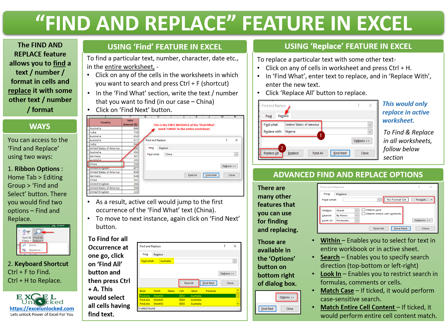
What if you are working in a big workbook with huge data in different worksheets and you want to find a particular text or a number and do something with it. In such a case, the Find and Replace Feature in Excel proves to be a life-saver for you.
Using the Find and Replace dialog box, you can find a specific text or a number in the worksheet or even the entire workbook. It is not only limited to finding a text or number, but you can also perform many advanced searches like finding something inside of the formulas or comments (instead of the cell content).
We would also unlock the technique to use wildcard characters with the Find and Replace features for advanced filtered searchings.
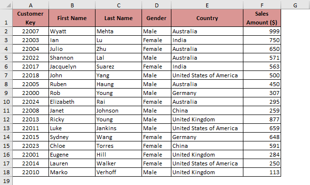
Sample Data
Below is the sample dataset table for Find and Replace Feature in Excel
Multiple Ways to Open ‘Find and Replace’ Dialog Box
There are many ways using which you can open the ‘Find and Replace’ dialog box.
Using Ribbon Options – You can navigate to the Find and Replace dialog box using the options available on the ribbon.
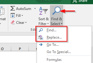
Go to Home Tab > Editing Group > ‘Find & Select’ button. In the drop-down options that appear, the first two you can see are the ‘Find’ and ‘Replace’ options.
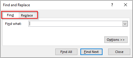
Both these options (Find and Replace) open the same dialog box named ‘Find and Replace’ dialog box. There are two tabs in it – one for ‘Find’ and another for ‘Replace’ as shown in the screenshot below:
Keyboard Shortcut – Another way to open the ‘Find and Replace’ dialog box, is by using the keyboard shortcuts. Use Ctrl + F for ‘Find’ and Ctrl + H for ‘Replace’.

Find Text or Number in Excel
Let us first learn how to use the Find and Replace dialog box to find text, numbers, dates, or other characters in Excel. Follow the below steps to achieve the same:
Also Read: How to Replace Values in Excel Power Query
To search across the entire worksheet, click on any of the cells in the worksheet and press Ctrl + F. As a result, the ‘Find and Replace’ dialog box would appear on your screen with ‘Find’ tab active.
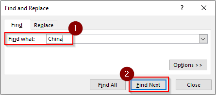
In the ‘Find What’ box, enter the text that you want to search for and click on the ‘Find Next’.
As a result, the excel selects the first instance of the ‘Find What’ text (China) in the active worksheet.
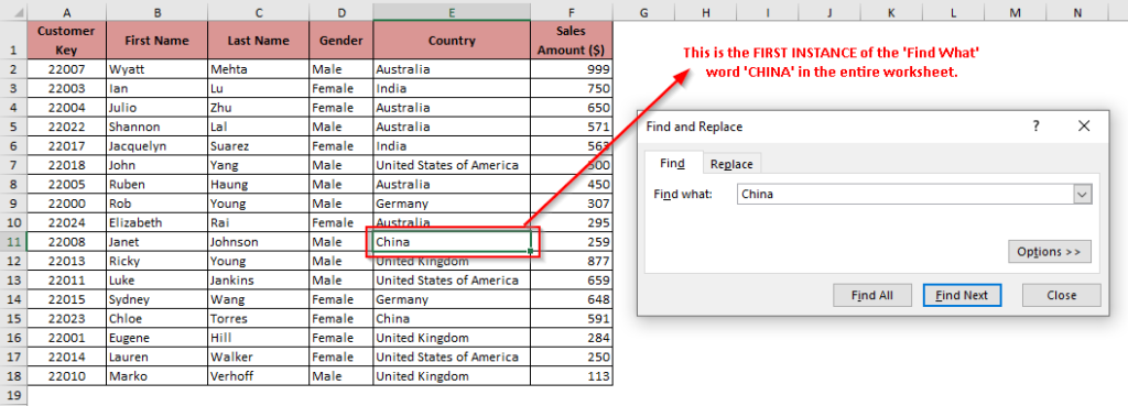
To find the next cell, again click on the ‘Find Next’ button and the active cell would jump the next instance of the word ‘China’.
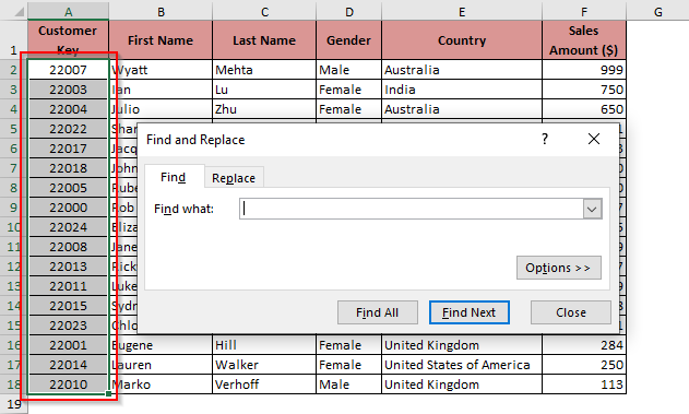
To find a specific text or number from a selected range of cells, select the cell ranges, and then use the ‘Find and Replace’ dialog box to find it.
As shown in the below image, the search would be limited to the selected cell range A2:A18.
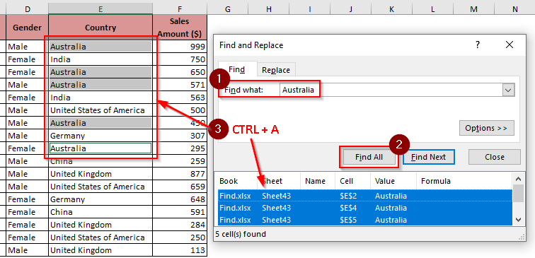
To find for all the instances, use the ‘Find All’ button. As a result, you would find the list of all the occurrences as shown in the below image.
Clicking on the occurrence in this list would take you to that cell.
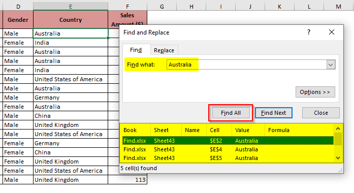
If you want to select all the cells that have the word ‘Australia’, just use Ctrl + A keyboard shortcut to select all the listed occurrences.
Using Advanced Find Features in Excel
You can also perform many other advanced finds using the extra options under the ‘Find’ tab.
To get more options to find, click on the ‘Options’ button under the ‘Find’ tab.
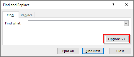
Some extra options would appear in this dialog box, as highlighted in the image below:
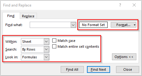
Let us understand each of these options
Within – By default, the excel only finds for the text or number in the active worksheet. To expand your search to the entire workbook, in the ‘Within’ drop-down box, select the option ‘Workbook’.

Search – This option allows you to choose for the direction of the search. If you choose – ‘By Rows’, then excel would search from top-bottom (i.e. one row after another) from the active cell (by default). You can change the direction to ‘By Columns’ to let excel search from left to right.

Look In – There are three options under this drop-down menu – Formulas, Values, and Comments. These options enable you to search for the search text, number, or characters inside comments or the formulas. Choose the valid option based on your need.

Match Case (Checkbox) – If you tick this checkbox, excel would do a case-sensitive search for the text that you enter in the ‘Find What’ input box. By default, Excel does not perform a case-sensitive search.
Match Entire Cell Content (Checkbox) – If this checkbox is ticked, the excel would find and select only those cells in which search text matches in its entirety (exact match of content in the cell).

Find Cells With Formatting
To find cells that contain specific formatting, follow the below steps:
Open the ‘Find and Replace’ using Ctrl+F keyboard shortcut and click on the ‘Options’ button (for more find options).
Besides the ‘Find What’ input box, you would find a button named ‘Format’ and click on it to open the ‘Format Cells’ dialog box.

In the ‘Format Cells’ dialog box that appears, search for the specific ‘Format’ that you want to find.
Alternatively, you can even use the ‘Choose Format From Cell’ to directly select the format from the cell itself.
As demonstrated in the image below, click on the option ‘Choose Format From Cell’. As a result, the mouse cursor would change to a plus symbol with a brush.
Now click on the cell containing the search format.
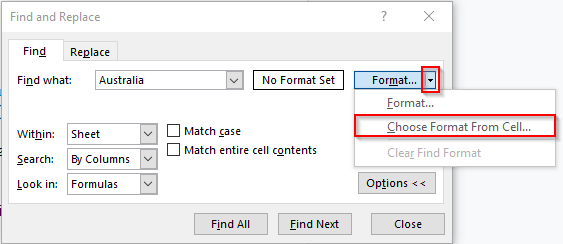
I quite often use this feature to search for all the cells that contain a specific fill color and replace all those colors with another color.
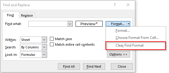
But, make sure to clear the formatting before going for any more searches. This is because Excel always saves the previously searched format. To clear the formatting, use the option ‘Clear Find Format’ as highlighted below:
Replace Text or Number in Excel
In this section, we would see how to replace a text, number, character, etc. To do this, we can use the ‘Replace’ tab of the ‘Find and Replace’ dialog box or use Ctrl + H keyboard shortcut to directly jump to the ‘Replace’ tab. It would help to replace one value with the other in the cells in Excel.
There are two input boxes in this tab – One is ‘Find What’ and another one is ‘Replace With’.
‘Find What’ – Here you need to enter the text that you want to find (to be replaced with something else).
‘Replace With’ – Here, you need to enter the replacement text.
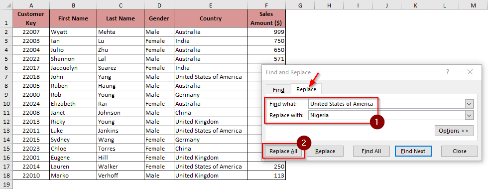
For example: let us replace all the cells having the country ‘United States of America’ with ‘Nigeria’. Follow the below steps:
Press Ctrl + H to open the ‘Find and Replace’, the ‘Replace’ tab would be the active tab by default.
In the ‘Find What’ section, enter the ‘United States of America’ and in the ‘Replace With’ section, enter ‘Nigeria’. Finally, click on the ‘Replace All’ button as shown in the below image-
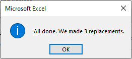
As a result, the excel would prompt a small window which says showing information about the total number of replacements made.
Click ‘OK’ and you would notice that Excel replaced the country name ‘United States of America’ with ‘Nigeria’ in all the cells in the selected worksheets.
To do the replacement only in the selected cell range, firstly, select the cell range and then use the ‘Find and Replace’ dialog box to replace.
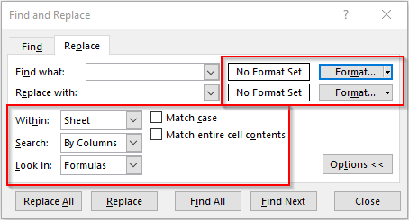
Additionally, just like the ‘Find’ options, you can perform advanced replace usings available options under the ‘Options’ button as highlighted in the image below.
Using Find And Replace With Line Break In Excel
The Find and Replace dialog box would be a life-saver tool when you want to insert or remove line breaks in excel.
Let us quickly go through the technique to insert a line break using the ‘Find and Replace’ option.
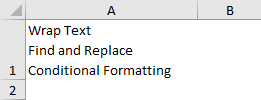
As you can see in the below image, the texts are written in cell A1 separated by a semi-colon (;). The purpose is to insert each of these texts in a new line in the same cell (A1) in Excel.

To achieve this, follow the below steps
Use Ctrl + H keyboard shortcut to open the ‘Find and Replace’ dialog box. In the ‘Find What’ section, enter the semi-colon sign (;) followed by a space, and in the ‘Replace With’ section, just press Ctrl + J.
Finally, click ‘Replace All’ button as shown in the image below:
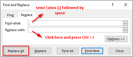
Ctrl + J is a shortcut key for a line break (newline in the same cell).
As a result, you can see that excel replaces the semi-colon (followed by space) with line break.
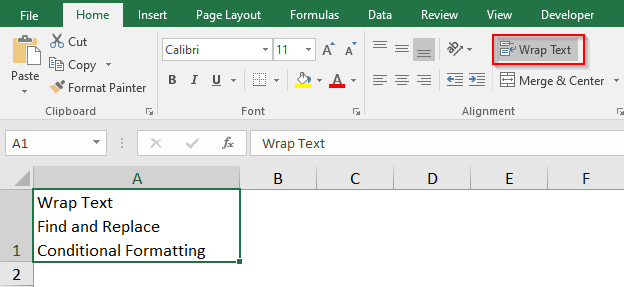
Make sure that the row width fits the cell content and wrap text button is on as shown in the screenshot below:
Using Find and Replace with Wildcard Characters
Wildcard characters are the special characters that are used for performing advanced filters and searches in Excel. There are three wildcard characters used in excel which are – Asterisk (*), Question Mark (?), and the Tilde (~). Wildcard characters are very useful when you want to create your own custom number format.
In a similar way, you can use the wild card characters with the ‘Find and Replace’ feature to perform advanced searches.
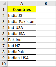
As you can see from the above image, the country combination for India and USA, is written inconsistently.
To replace all the cells having inconsistently written India and USA and replace it with a specific text like ‘India-USA’, we can use the ‘Find and Replace’ feature along with the wildcard characters.
Use keyboard shortcut Ctrl + H to open the ‘Find and Replace’ dialog box. In the ‘Find What’ section, enter *Ind*US*. And in the ‘Replace With’ section, write the replacement text India-USA.
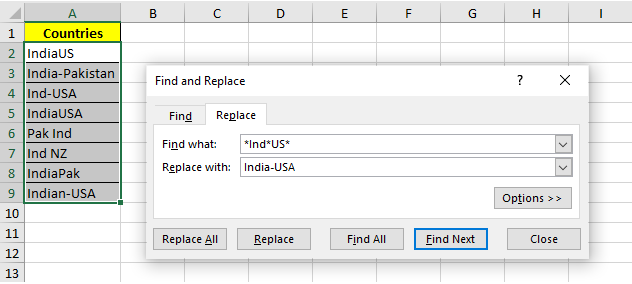
The Asterisk symbol in the text *Ind*US* denotes any number of characters before the word Ind, in between the words Ind and US and after the word the US. To learn more about ‘Wildcard Characters in excel’, click here.
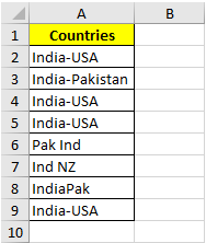
As a result, the excel would search for Ind and US texts and replace it with India-USA as shown in the screenshot below:
This brings us to the end of this blog. Share your views and comments in the comment section below.

