In one of our previous blogs, we learned how to use the =VLOOKUP() function for Partial Match in Excel. To explore it, follow our previous blog on “Using =VLOOKUP() Function for Partial Match in Excel“. In this blog, we would explore and unlock the technique to use the =IF() function for a partial match in Excel. Many a time, you have an excel worksheet where you want to use the =IF() function in such a way that it should return the values even for a partial match of string in Excel.
Let us take a look into what this blog would help you to achieve.
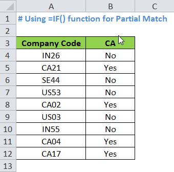
In the below screenshot, you can see that there is a list of company codes that starts with the country code followed by a two-digit number.
You now want to search for the company codes located in a specific country (let’s suppose in Canada).

Let us now begin with this technique.
The formula for Using =IF() Function for Partial Match
Enter the following formula in cell B4:
=IF(ISNUMBER(SEARCH($B$3,A4)),”Yes”,”No”)

Press the “Enter” key on your keyboard. As a result, you would notice that excel returns the value as “No” as the company code IN26 does not belong to Canada(CA).
Copy the cell B4 using Ctrl+C shortcut in your keyboard and paste it to the other cells in column B.

Now, let us understand each of the components of this complex formula one by one to know how this formula actually works.

Explanation of Formula
There are mainly three formulas that are used to achieve this. The first one is SEARCH formula, the next one is ISNUMBER and the last one is IF formula.
Let us explore each of these formulas one by one.
The SEARCH Formula
This formula returns the position of a text in the search string. In the present case, it would search for the value in cell B3 and return its position in A4.
Thus, the excel would search for the text “CA” in the company code list and return its position. If it finds the text “CA”, then it would return the value as “1” (as the text CA is positioned at the very beginning of each of the search string company codes).
The ISNUMBER Formula
This formula returns the value as TRUE if the reference cell value is a number. And it would return FALSE, where the reference cell value is not a number.
The SEARCH formula is inside the formula ISNUMBER. The SEARCH formula returns TRUE if it is a number, else would return FALSE.
In the present case, where ever, the excel finds the word “CA” in the company code, it would return “1”, and as 1 is a number, the ISNUMBER formula would give “TRUE” for those company-codes.
The IF Formula
The IF function can perform a logical test. It returns one value for a TRUE result and another for a FALSE result.
The IF function checks the condition entered in the first attribute and returns the value specified in the second attribute if the condition is fulfilled or returns the third attribute if the condition fails.
In our case, the first attribute of the IF function is ISNUMBER(SEARCH($B$3,A4)) and the second and third attributes are “YES” and “NO”.
This means that if the value of the ISNUMBER(SEARCH($B$3,A4)) is TRUE, the excel would return the value as “YES” (the second attribute of IF formula) and “NO” if it is FALSE.
Some More Testing
Now let us change the country and check how does this formula behaves.
Let us now check for the company codes in the United States(US). Enter the text “US” in cell B3 and press Enter.
Consequently, the excel would enter “YES” in front of the US Company Codes and “NO” in front of others.
This brings us to the end of this blog. Share your comments and view on this blog in the comment section below.