AutoFit Column Width and Row Height in Excel

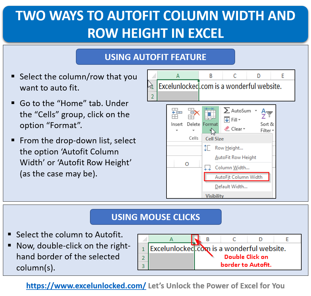
This amazing blog aims at unlocking various techniques to AutoFit the row height and column width of Rows and Column in Excel. There are various methods available in Excel using which you can AutoFit the row height and column width in Excel.

Before you change the row height and column width in Excel, let us first understand what is the default setting.

Default Row Height and Column Width in Excel

Whenever you open any new excel workbook, the default row height and column width are 15 and 8.43 respectively. This corresponds to 64 pixels (for row height) and 20 pixels (for column width).

You can validate the same by using the below procedure.

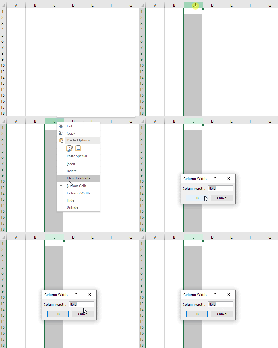
Open any new excel worksheet. To check the row height of the cells, right-click on any of the row headings and select the option “Row Height”.

You would notice that the “Row Height” dialog box would appear. It shows 15 as the row height.

Similarly, you can check the column width by right-clicking on any of the column headings and selecting the option “Column Width”.

Amazing Facts about Row Height and Column Width

The minimum row height and column width are 0 (zero). This represents the hidden column or row in Excel. The Zero width and height are just like Hidden columns and rows in Excel.

The maximum column width can be 255. Similarly, the maximum row height can be 409.

Using Excel’s AutoFit Feature

Let us now begin with learning the amazing AutoFit feature in Excel.

Suppose that you have a text written in cell A1 in Excel which extends beyond the default column width. 

You would notice that the text would flow beyond the cell A1 and overlap the adjacent cell(s).

Look at the image below:

Similarly, you can see in the below screenshot that the text moves out of the row height and is not visible completely.

To adjust the column width and row height, you can use any of the below methods. 

The first one is by using the option on Excel Ribbon. And the other one is by mouse-click.

Let us take a look at each of the methods one by one.

Method 1: Using AutoFit Options on Excel Ribbon

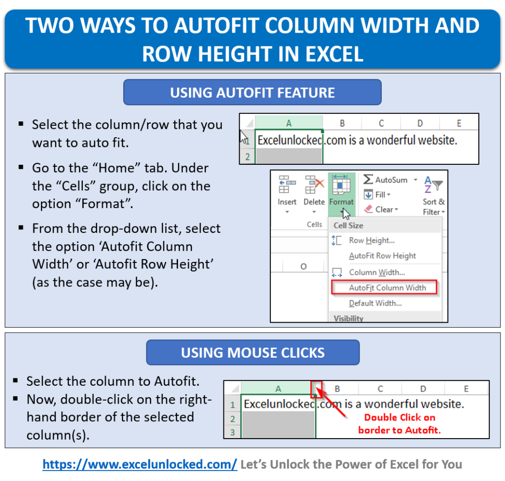
To AutoFit Columns Width and Row Height in Excel, follow the below steps:

Select the column that you want to AutoFit. In the present case, I have selected column A.

Go to the “Home” tab. Under the “Cells” group, click on the option “Format” as shown in the screenshot below:

The drop-down options would appear. Select the option “AutoFit Column Width”.

This brings us to the end of this blog. Share your views and comments on this blog in the comment section below.

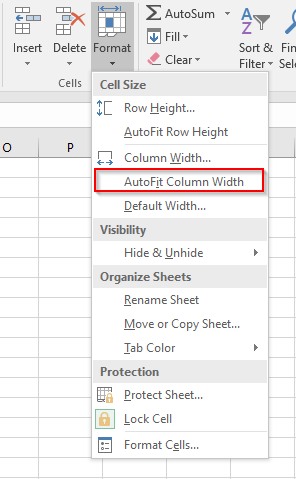
You can see that the column fits itself to occupy the entire sentence in cell A1.

Similarly, to AutoFit the Row Height, select the row and navigate to the “Format” option in the ribbon and click on the option “AutoFit Row Height”.

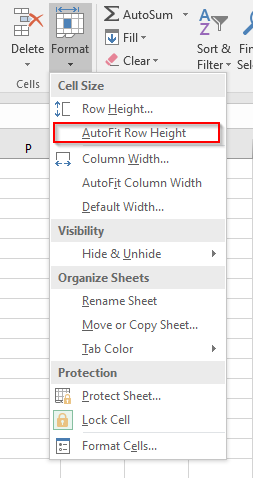
As a result, you would notice that the height of the selected row adjusts itself according to the height of the content in the cell.

Method 2: Using Mouse Clicks

Instead of using the above method, you can even use the other simpler method to AutoFit the Column Width and Row Height to fit the cell content.

Simply select the column(s). Now, double-click on the right-hand border of the selected column(s).

Refer to the picture below:

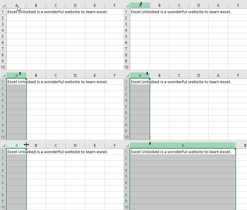
Finally, you can see that the excel column fits itself to the content length.

Similarly, select the row(s) and double-click on the bottom boundary of any of the selected row(s).

This brings us to the end of this blog.