Do you know how to wrap a text in an excel cell? What is the purpose of Wrap text function in excel?
Many a time while writing some text in an excel cell, it happens that the text crosses the cell width and overlaps the content existing in the adjacent cell. As a result, the content in the adjacent cell disappears.
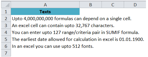
Below is the example wherein you can see that text in column A overflows to cells in column B and even up to columns C and D.
Do you know what solution has excel provided for this?
To solve this issue, excel has an embedded functionality to wrap the text.
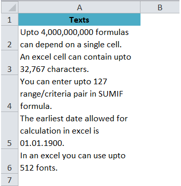
WRAP TEXT: Wrap Text feature in excel makes sure that the text in an excel cell is confined within that cell only and does not overlap/overflow to the adjacent cells. Any text beyond the cell column width moves to the next line in the same cell as shown in the screenshot below :
Also Read: Wrap Text Using VBA – Examples
There are various ways in which you can use the Wrap text functionality of Excel.
- Wrap Text using a single click
- Using Keyboard Shortcut
- Wrap Text using Format Dialog Box
- Wrap Text using the line break
Let us understand each of the methods in detail to have a complete understanding of this functionality:
Using a Single Mouse Click
Being an often-used functionality, Excel has provided this functionality on the face of the excel worksheet, so that it is easy to access the same.
Refer to the data below. As you can see that the data in the cells overflow to the adjacent cells.
Now, you want to fit the content in the respective cells.

To achieve the same, follow the below steps :
Step 1 : Select the text in column A.
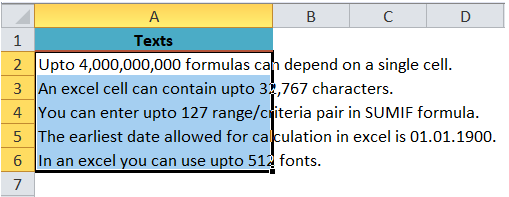
Step 2 : In the ribbon bar, click on the tab ‘Home’. Under the “Alignment” group, click on the option “Wrap Text” as highlighted in the screenshot below :

As soon as you click on the “Wrap Text” icon, you would see that excel wrapped the text in the selected cell.
Also Read: AutoFit Column Width and Row Height in Excel

Using Keyboard Shortcut
You can even use the keyboard shortcut to wrap the text in Excel. It would make your task faster.
Select the text and press the Alter key on your keyboard followed by “H” and then “W” (i.e. Alt + H + W).
You can see that all the selected text fits to the column width.
Wrap Text using Format Dialog Box
You can use also use this method to wrap a text in an excel cell.
Follow the below steps :
Step 1 : Select the cells on which you want to apply wrap text formatting.
Step 2 : Click on the “Home” tab. Under the “Alignment” group, click on the dialog box launcher (a small arrow like symbol at the bottom right of the “Alignment” group) as highlighted in the screenshot below :

The “Format Cell” dialog box will open.
Step 3 : Now tick the checkbox “Wrap Text” under the “Text Control” section and then click on OK as shown in the screenshot below.
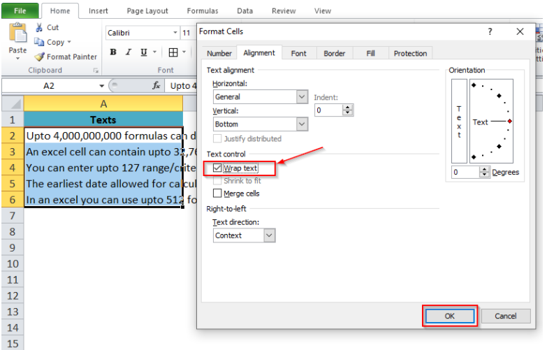
If you see the original sample data, you can see that the selected text fits to the column width.
Wrap Text using line break manually
When you apply wrap text into any cell, the text in that cell fits the column width of that cell.
Where the length of the text is less than the column width, in such case, the text will not wrap (and is as such not required). But if the length of the text in excel cell exceeds the width of the cell, then the Excel would break the text up to the width of the cell and take the remaining text to the second line in the same cell (and so on).
However, using this keyboard shortcut trick you can also put a line break manually. This would break the line and take the remaining text to the second line.
Follow the below procedure to manually put a line break :
Step 1 : Double click on the cell in which you want to insert a line break.
Step 2 : Now place your cursor at the place in the text where you want to have a line break.
For example, in a text in cell A2, I want to put a line break after the word 4,000,000,000. In that case, I need to put my cursor after the word 4,000,000,000 as shown in the screenshot below.
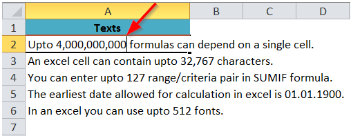
Step 3 : Now press Alt + Enter key on your keyboard.
You can see that as soon as you press Alt + Enter, the excel took the remaining text to the second line within the same cell.
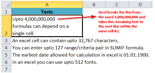
You can try the same with some other cell content. Let’s take cell A4. Follow the above steps to break the line from the word “upto”.
With this you have reached to the end of this blog. Share your views and comments in the comment section below.

