VLOOKUP Function Returning Multiple Values

VLOOKUP Function is a type of most used and important lookup function. It has a wonderful functionality, In this blog, we will see the VLOOKUP Function returning multiple values and working as an array formula. We will learn how to look for multiple parameters of a single entity.

So let’s start implementing this critical application of the VLOOKUP Function.

Revising the Concept of VLOOKUP Function

Before we actually start implementing the application of the VLOOKUP Function, let’s brush up on the function basics with a few lines.

=VLOOKUP(lookup_value,table_array,col_index_num,[range_lookup])

• The VLOOKUP Function searches for particular information regarding an entity.
• The Formula first looks for the lookup value in the first column of table_array.
• If the search is successful, then the function returns a value corresponding to the lookup_value in the column specified by the col_index_num
• [range_lookup] is an optional argument and asks for an exact or approximate match.

Example 1 – VLOOKUP Function Returning Single Value

In this example, let us suppose we have the details of different students of a class as follows.

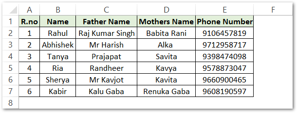
We have five columns containing the Roll Number, Name, Father Name, Mother Name and Phone Number of the student. In this data, every student has a unique roll number. Therefore, we can look for student information with the help of its roll number.

Let us suppose we want to get the Phone Number of Students having Roll Number 5. You can simply check this information as we have records of 6 students only. We can use VLOOKUP Function when there are a number of records having multiple columns.

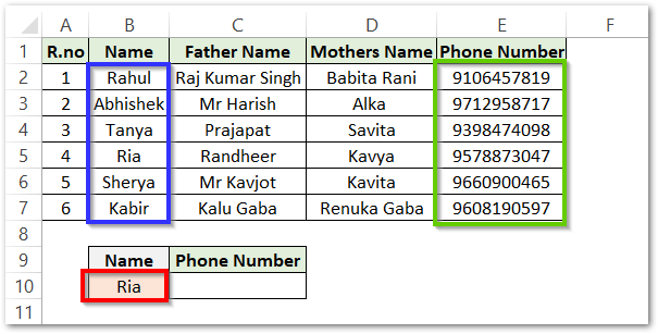
Here the Name in the red box is the student name whose phone number we want to get. Blue Box contains the name of the students while the green box has their corresponding Phone Number.

Use the following formula in cell C10 to get the Phone Number of Ria from the student records.

=VLOOKUP(B10,B2:E7,4,0)

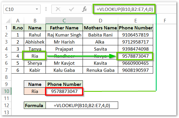
As a result, the VLOOKUP Function has returned the Phone Number of Ria as 9578873047.

Explanation – We have passed the lookup value as cell B10 which has the name, Ria. The Name Ria is searched in the first column (B) of the table_array B2:E7. The value corresponding to Ria in the 4th column (E) ( supplied as col_index_num ) is Ria’s Phone Number. Consequently, the formula returns the results.

Example 2 – VLOOKUP Function returning Multiple Values

VLOOKUP Function can work as a dynamic array function ( For excel 365 ) and as a CSE ( array formula for all versions of excel ). The Function can return an array of values as its result.

This case is possible when we want to extract multiple information parameters about one entity from a range of data.

Let us suppose we want to extract the entire record of Tanya from the above data.

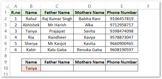
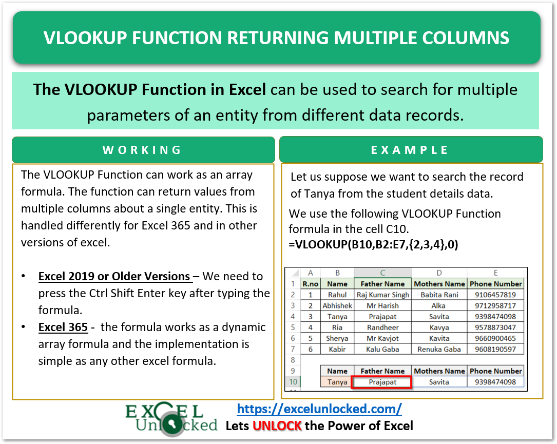
Here, we want to find the record of Tanya highlighted in Red. Type the following formula in cell C10 and press the Ctrl Shift Enter key after typing this formula.

=VLOOKUP(B10,B2:E7,{2,3,4},0)

We type the formula in cell C10, once you hit the Ctrl Shift Enter key, the function results are automatically spilled into the array of cells C10:E10.

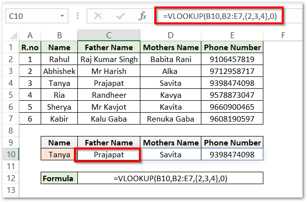
As a result, we get complete information about Tanya.

Explanation – This time, we have used the VLOOKUP Function as an array function. We have passed the lookup_value argument as cell C10 which has the name we are searching for. table_array is the same as in the previous example, B2:E7.

The third argument col_index_num is supplied with an array of column numbers separated with commas, {2,3,4}. This is so because, we wanted the corresponding parameters from the 2nd (Column C ), 3rd ( Column D ) as well as 4th ( Column E ) column of the table_array.

0 is for exact_match.

So we have now seen the VLOOKUP Function returning multiple values.

This brings us to the end of the blog.

Thank you for reading.