Dynamic Array Formulas are real game changers when one knows how to use them! They are compatible with Microsoft Excel 365 and Excel 2022 versions. Dynamic Array Formulas have added the most incredible functioning to excel formulas and functions.
Let us see how they work!
What are Dynamic Array Formulas?
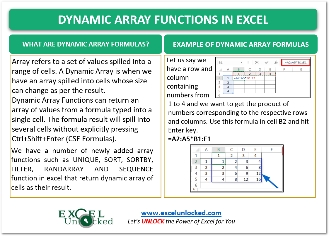
Array refers to a set of homogenous values. A Dynamic Array is when we have an array spilled into cells whose size can change as per the result.
Dynamic Array Functions can return an array of values from a formula typed into a single cell. The formula result will spill into several cells without explicitly pressing Ctrl+Shift+Enter (CSE Formulas).
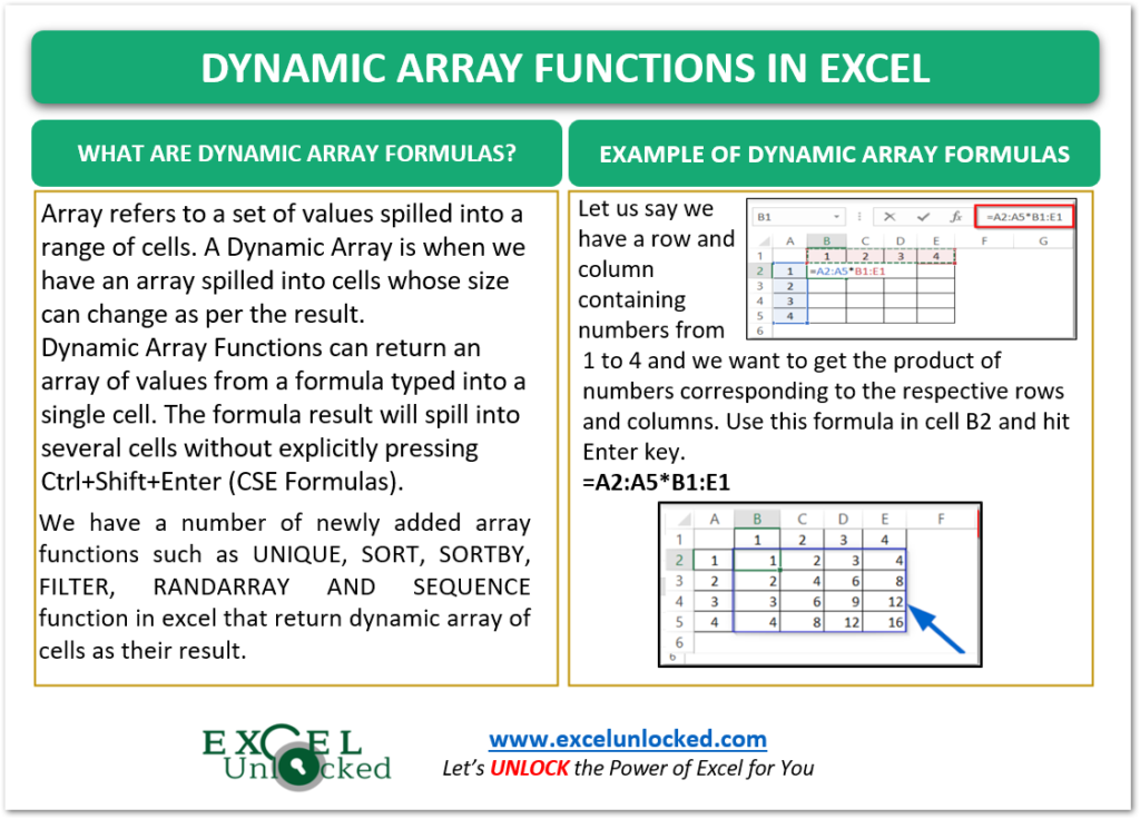
Let’s take an example. We have entered the following dynamic array formula in cell B2.
=A2:A5*B1:E1
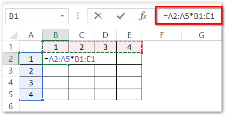
Once you type the formula in cell B2, hit the enter key. Consequently, you will see that the formula results have been split into the range B2:E5.
Also Read: SORT Function in Excel – Usage with Examples
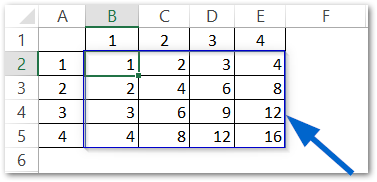
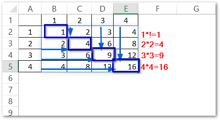
The formula has returned the product of the cells in the corresponding rows and columns.
List of Newly Introduced Dynamic Array Functions
Here we have some of the functions that return ranges based on the Dynamic Function we use.
- UNIQUE – Dynamically gives a range of unique values from the source range.
- SORT – Sorts the range of values in ascending or descending order.
- SORTBY – Sorts values based on a corresponding range
- FILTER – Filters a range based on the provided criteria
- RANDARRAY – Returns an array of random numbers between 0 and 1
- SEQUENCE – Generates a list of sequential numbers such as 1, 2, 3, 4, 5
Example 1 – One Cell, One Formula but Multiple Results
In this example, let us say we have the student names in the range A2:A8 as follows:-
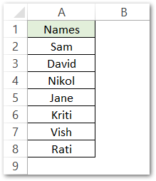
We want to sort these names alphabetically. To do this, we can use the SORT Function in Excel which is a dynamic array function.
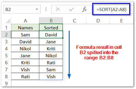
Use the following formula in cell B2.
=SORT(A2:A8)
As a result, the formula returns an array of names in alphabetically sorted order as follows:-
How to Refer to Spilled range in other Formulas
The reference to normal ranges is easy as all the cells are referred to by that range. But when we have a single formula, whose result makes up a spilled range, then the situation is different. We need to use an # after the cell reference (B2 in Example 1) which contains the dynamic array formula.
For instance, look at this example where we want to count the total number of cells in the spilled range by using the COUNTA Function of Excel.
Here we have the List of Departments containing Duplicates in cells A7, A8, and A9. We would now use the UNIQUE Function of Excel to get the Unique list of departments. Enter this formula in cell C2.
Also Read: Dynamic Named Range – OFFSET and COUNTA
=UNIQUE(A2:A9)
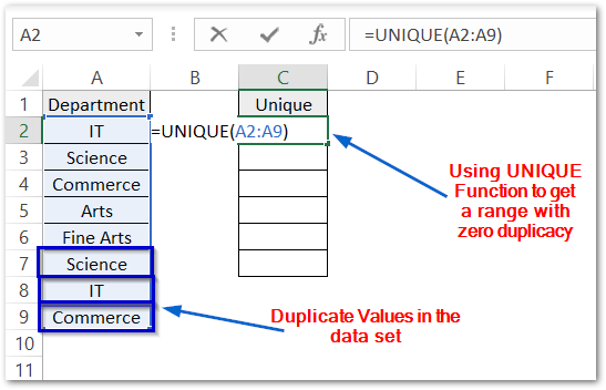
As a result, the result will spill dynamically to give a unique list of departments.
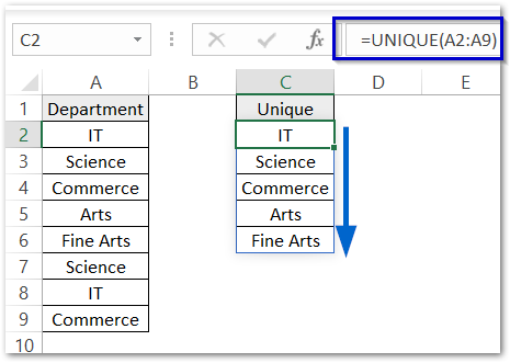
Now the spilled range is C2:C6. We would use the cell at the upper left corner of the range followed by # to refer to this spilled range.
=COUNTA(C2#)
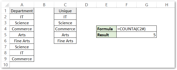
As a result, the formula returns 5 which means that there is a total of five departments.
How to resolve #SPILL Error?
A common error comes while using the dynamic array formulas which is a #SPILL error. The name of the error tells that this occurs when the formula result can’t spill and there is some problem with space. Any cell in the range that the formula would spill, is nonempty. For instance:-
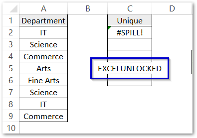
So you see that cell C5 is not a blank cell anymore and cell C2 shows a #SPILL error as the range in which the formula result was about to tp spill is no longer empty.
Make sure that the cells are blank and then the #SPILL error is removed. This is how we use dynamic array formulas in excel.
This brings us to the end of the blog.
Thank you for reading.

