FILTER Function in Excel – Dynamic Filtered Range

In the previous blog, we did some of the Dynamic Array Functions like the UNIQUE and SORT Function of Excel. The FILTER function in excel is also a new and advanced Dynamic Array Function that has gifted a new functionality to filter a range of cells based on certain criteria.

Let us see how the FILTER function works.

When to use FILTER Function in Excel?

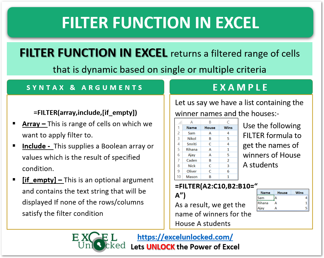
As the name FILTER suggests, the FILTER Function of excel returns a filtered range of cells that is dynamic ( size can be changed as per source ) based on one or multiple criteria. The result of the FILTER function automatically spills into a range of cells.

Only the values that meet the condition specified by the FILTER Function are allowed to be filtered and shown separately from the source range.

Syntax and Arguments

=FILTER(array,include,[if_empty])

Where the following are the required function arguments to use the FILTER function:-

• array – This is our source range from which we want to get the filtered results. It can be a reference to a range of cells or any function that returns a range of cells.
• include – In this argument, we specify the criteria that will be the base for filtering our array. The criteria return an array of TRUE and FALSE values whose size must be equal to the width or length of the array.
• [if_empty] – This is an optional argument and is not mandatory to specify. It is the value returned by the FILTER function if none of the rows satisfy the condition specified by the FILTER function.

Examples to Learn FILTER Function of Excel

In this section, we will perform some practical examples to learn the usage of the FILTER function.

Example 1 – Simplest Example to learn FILTER formula

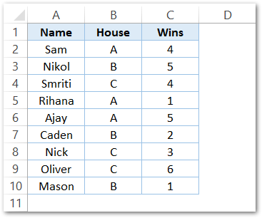
Let us suppose we have a list containing the names of winners, their houses, and the number of wins of each winner as follows:-

We want to filter the winner records for house A students. Assign a cell (F1 to contain “A”) to contain the house for which we want to get the records and Use the following FILTER formula:-

=FILTER(A2:C10,B2:B10=F1)

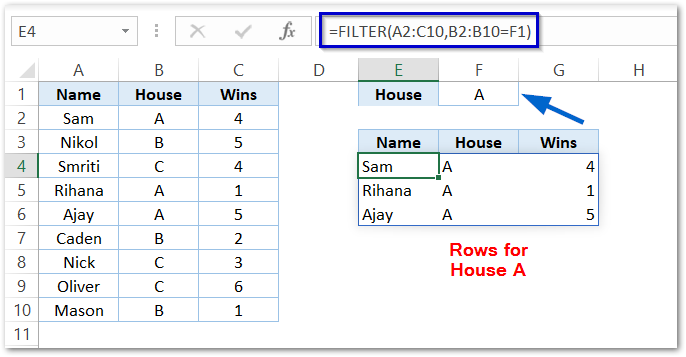
We entered the formula in cell E4. As a result, the rows for the House A winners filter out and spill into the range E4:G6.

Explanation – We have passed the range A2:C10 as our source range (array) to filter the results. Thereafter, in the include argument, we entered that the range B2:B10 ( containing houses ) must be equal to cell F1 ( containing house A ).

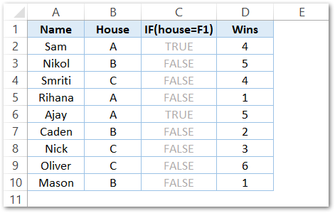
The include argument returns the list of boolean values. The rows corresponding to which the boolean value is TRUE ( for which the house = A ), are returned by the FILTER function.

Example 2 – FILTER Function with AND logic

Let us suppose that we want to apply the filter on our range such that the results must satisfy two conditions. This is when we can use the AND logic ( operator = * ).

We are taking the following list of winners. We want to filter those winners of House B that won exactly one time.

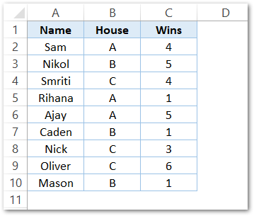
Use the following FILTER formula to get the required results.

=FILTER(A2:C10,(B2:B10="B")*(C2:C10=1))

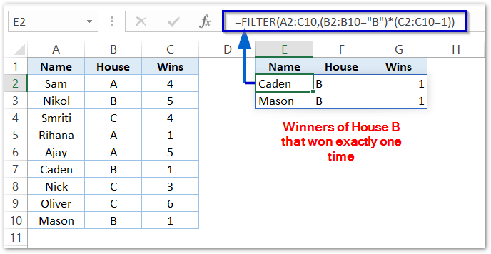
As a result, the formula has returned the records of winners for which the number of wins is 1.

Explanation – We have passed the range A2:C10 as an array argument so it will be the source range.

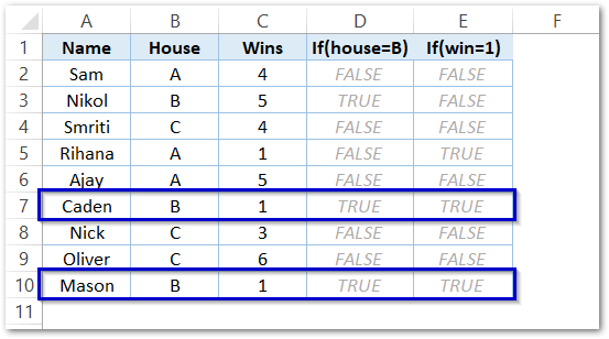
In the include argument, we have specified two conditions B2:B10=”B” ( house must be B ) and (*) C2:C10=1 ( number of wins must be 1). The include argument returns two boolean arrays with AND logic in between them.

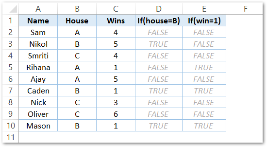
These are two boolean arrays in ranges D2:D10 and E2:E10. The rows for which both the values are TRUE, filter out.

Example 3 – Usage of if_empty Argument

Let us say we want to filter the records of house D students from the above source range. Use the following formula:-

=FILTER(A2:C10,B2:B10="D")

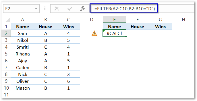
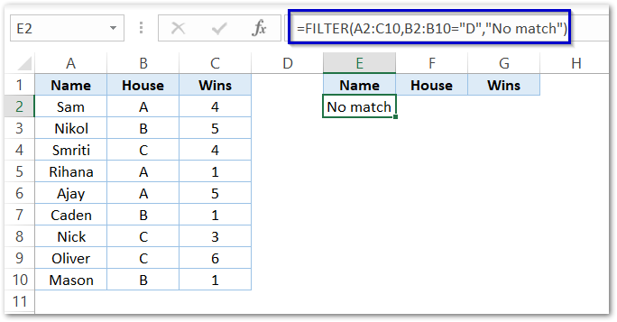
As a result, the formula returns a #CALC! error as there is no winner in House D. We can use the if_empty argument to display some other message when no entry matches the filter criteria.

=FILTER(A2:C10,B2:B10="D","No match")

You can extend your learning beyond this by going through some of the advanced applications of the FILTER Function.

This brings us to the end of the blog.

Thank you for reading.