Applications – FILTER Function in Excel

In the previous blog, we did the basic usage of the FILTER function in Excel. In this blog, we will learn some of the most practical usages of the FILTER function. The functionality of the FILTER formula increases a lot more when we merge it with other functions. So let’s start learning about the Applications of FILTER Function in Excel.

How to Filter Duplicates using FILTER Function

With the use of the FILTER function along with the COUNTIFS function, we can get those rows filtered out whose count in the source range is more than one ( have duplicates ).

Let us suppose that we have the following list of orders from a cookie company as follows:-

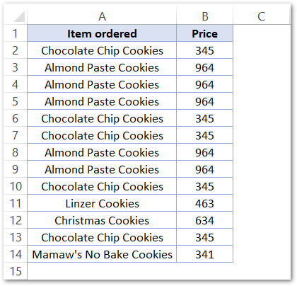
We want to see the duplicate orders placed from this list. Use the following formula in cell D2:-

=FILTER(A2:B14,COUNTIFS(A2:A14,A2:A14,B2:B14,B2:B14)>1)

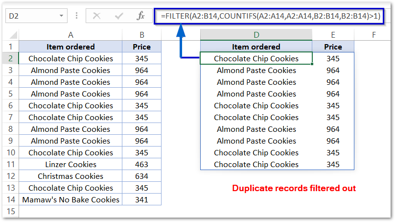
As a result, you can see that the FILTER function has successfully filtered the duplicate records.

The syntax to use this formula is:-

=FILTER(source_range,COUNTIFS(column1,column1,column2,column2.......columnN,columnN)>1)

Where the maximum number of columns in the COUNTIFS Function is N.

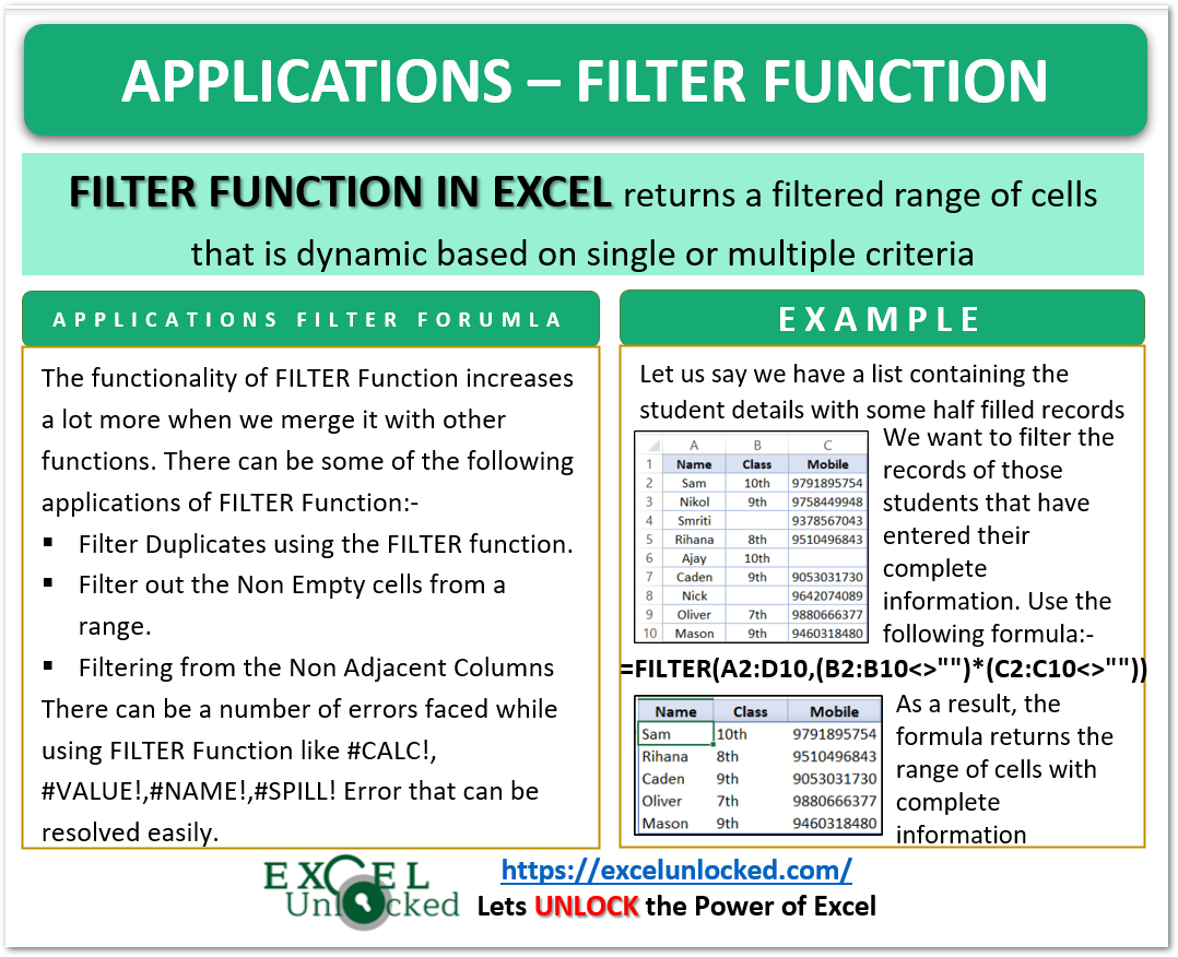
How to Filter out Non-Empty Rows in Excel?

In this section of the blog, we will learn how we can filter out the nonempty rows ( having no missing values) from our source range that contains blank cells.

Let us suppose we have the student information list as follows:-

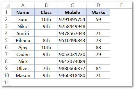
You can see in this list that some of the student details are missing.

Let us say we want to get the student details for those students who have submitted all of their details ( Class, Mobile, and Marks ).

Use the following formula in cell F2.

=FILTER(A2:D10,(B2:B10<>"")*(C2:C10<>"")*(D2:D10<>""))

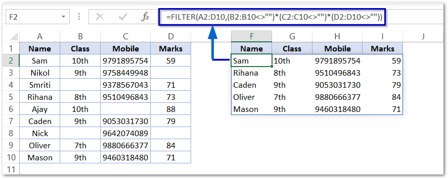
As a result, you will see that the students with complete information filter out.

We have applied the condition in the FILTER function that none of the Columns for Class, Mobile, and Marks should be a blank cell to be filtered out.

Filtering from Non-Adjacent Columns

We can filter our data by picking up those columns that are not adjacent to each other by using the Nested FILTER ( FILTER on FILTER ).

Here we have the Order Details, Prices, and Order IDs.

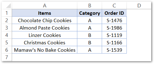
Let us suppose we want to filter the Items from Category A but we only need the item Names and Order Ids. Use the following FILTER formula:-

=FILTER(FILTER(A2:C6,B2:B6="A"),{1,0,1})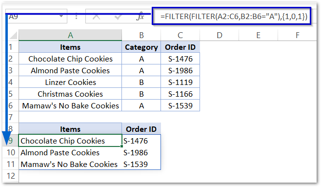

As a result, the formula has returned Item Names and Order Ids as we had applied a filter to get the first and last column ({1,0,1}).

We can have many more Applications of FILTER Function in Excel as per our requirement.

Errors to Resolve in FILTER Function

While using the FILTER function, you might face the error messages returned instead of the required results. Following are the error messages, their meanings, and how we can resolve them.

#CALC! Error

Whenever we specify the criteria ( include ) that none of the entries in our source range meets, then we get the #CALC! error. We can resolve this error by mentioning the if_empty argument.

#VALUE Error

This error occurs when the size of the boolean array returned by the include argument does not have a size equal to that of the array dimensions. We need to change

#NAME! Error

The FILTER Function is compatible with Excel 365 and Excel 2022. In older versions, it returns a #NAME! error.

#SPILL! Error

This error occurs when the FILTER Function resultant range does not get enough empty range of cells to spill. WE need to empty the cells covered under that area and the error is resolved.

This brings us to the end of the blog.

Thank you for reading.