Using =VLOOKUP() Function for Partial Match in Excel

Many times you have excel data where you want to do a partial match of the data. To perform a partial match of data in Excel, we can use =VLOOKUP() function along with the wildcard characters.

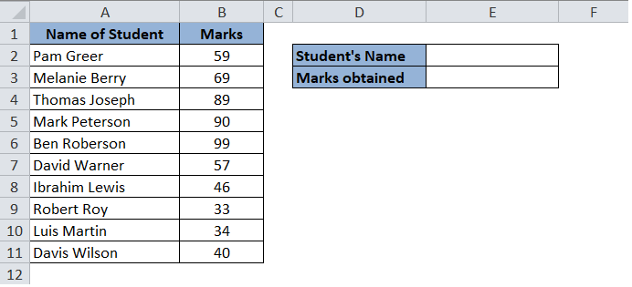
Let’s say you have a data table in excel. This data contains student’s full names in one column and their marks in another column.

Now, you want that when you enter the first name in cell E2, the Excel should automatically populate the marks obtained in cell E3.

This could have been easily done using a simple =VLOOKUP() function in excel if in case there is an exact name (exactly the same as mentioned in the marks table) in cell E2.

In this blog, we would learn how to auto-populate the marks in cell E3 if we just enter the first name or the last name of the student in cell E2.

This can not be done using simple excel =VLOOKUP() functionality. =VLOOKUP() formula would be used along with wildcard characters to achieve the same

Let us begin with this tutorial.

Partial Match Using Formula

Enter the following formula in cell E3 :

=VLOOKUP(E2&”*”,$A$2:$B$11,2,FALSE)

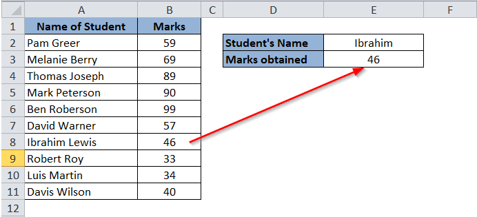
Now, try entering the first name of any of the students in cell E2 (let us suppose we enter Ibrahim). As soon as you press the “Enter” key on your keyboard, you would notice that the cell E3 gets filled with the marks obtained by Ibrahim (from the marks table).

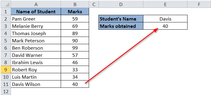
Now change the name of the student in cell E2 and then check the value in cell E3. 

Similarly, to get the marks obtained by a student based on his last name, use below formula-

=VLOOKUP(”*”&E2,$A$2:$B$11,2,FALSE)

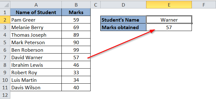
Now, enter any last name and as a result, you would get respective marks obtained based on the last name.

Explanation of the Formula

In the present case, we are supplying the first attribute of the =VLOOKUP() formula as E2&”*” (i.e. the value to lookup followed by an asterisk sign). The “&” operator in between the text E2 and asterisk symbol concatenates (combines) the text E2 and asterisk symbol (resulting in as E2*). 

This denotes that the excel should search for the text that starts with the value specified in cell E2.

Similarly mentioning “*”&E2 as a first attribute denotes that excel should search for the text that ends with the value specified in the cell E2.

The second attribute of the formula is the data range where the excel would search for E2* or *E2. In the present case, our data range (lookup range) is A2:B11.

The third attribute in the formula is “2”, which denotes that excel should return the value specified in the second column of the selected data range (lookup range).

The fourth attribute of the formula is FALSE. This means excel should search for an exact match and not an appropriate match.

Precautions To Be Taken

However, this formula would not work when there are two students with the same first name. 

For example, when you have two students, one with the name “John” and another “Johnson”. In this case, when you type the word “Joh” in cell E2, excel would return the value that occurs first in the selected data table.

I hope you have enjoyed learning this technique of finding a partial match. Practice this with different data sets. Share your comments and thoughts in the comment section below.