It is elementary to design a calendar in excel in just three steps. We can make the calendar using the SEQUENCE Function. We would use formulas containing functions like EOMONTH, CHOOSE, SEQUENCE, DATE, WEEKDAY, and conditional formatting.
It is assumed you understand the basic functioning of these topics. If you do not have prior knowledge of any of these functions, then it is highly recommended to learn their basic usage as making the calender would involve it.
Calendar Using Sequence Function
The Calendar we are about to make would input the month and year from the user and then show the corresponding calendar for that month of the specified year.
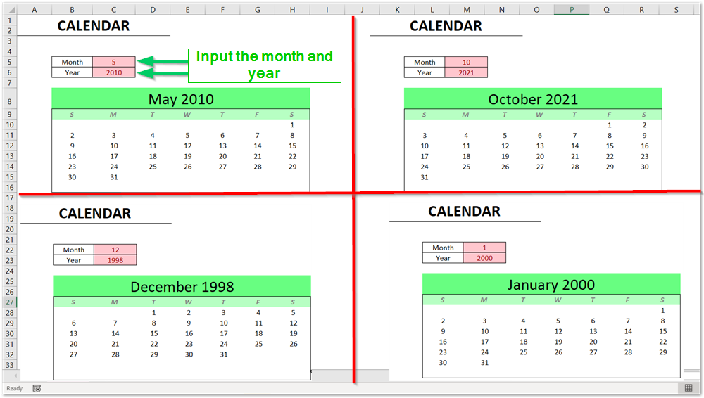
We can change the value in input cells for month and year and this calendar is going to automatically update itself.
Since we already mentioned that making this calendar involves three steps. These steps are as follows.
- preparing input cells
- writing formulas
- formatting
You can have the practice workbook to work along this article.
Step 1 – Preparing Input Cells
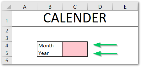
We need to have two input cells, one is for specifying month and another is for specified year. We can apply different cell styles to make them look different.

Select the Red cell style for inputs.
Step 2 – Applying Formulas
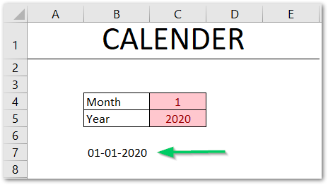
We would now use the following formula in cell B7.
=DATE(C5,C4,1)
This would return the first day of the month and year specified in the input cells.
Now use the following formula in cell B9.
=SEQUENCE(6,7,CHOOSE(WEEKDAY(B7),1,0,-1,-2,-3,-4,-5))
Note that we have written the labels for Weekday in the 8th row as S, M, T, W, T, F, S
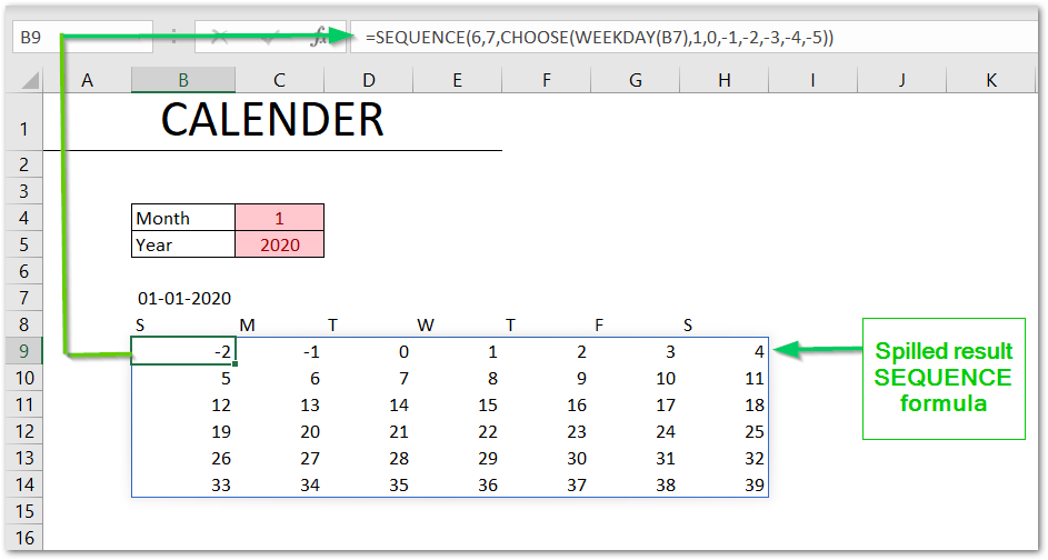
Explanation – The result of the sequence function is spilled in the range B9:H14. We have used the SEQUENCE Function to get the sequence of numbers. The rows and columns argument is hard coded as 6 rows and 7 columns ( for all weekdays ). The start argument is optional in the SEQUENCE Function and we have made the starting number in cell B9 dynamic using this formula.
CHOOSE(WEEKDAY(B7),1,0,-1,-2,-3,-4,-5)
This starting number would define on which day the 1st of each month in the calendar would lie. If the weekday of the first of that month is Monday, then 1 must come in cell C9 and the starting number is 0.
| Weekday on the 1st of the month | 1st of the month lies in the cell | Value in cell B8 |
| Sunday | B9 | 1 |
| Monday | C9 | 0 |
| Tuesday | D9 | -1 |
| Wednesday | E9 | -2 |
| Thursday | F9 | -3 |
| Friday | G9 | -4 |
| Saturday | H9 | -5 |
Step 3 – Applying Formatting
We would now apply two conditional formatting rules in order to hide the negative value of days and the invalid days.

Hiding these irrelevant dates is mandatory in a calendar. To do so, we would use two conditional formatting rules.
- Select the range B9:H14.
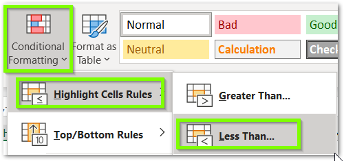
- Click on the Conditional Formatting button and go to the Less Than formatting rule.
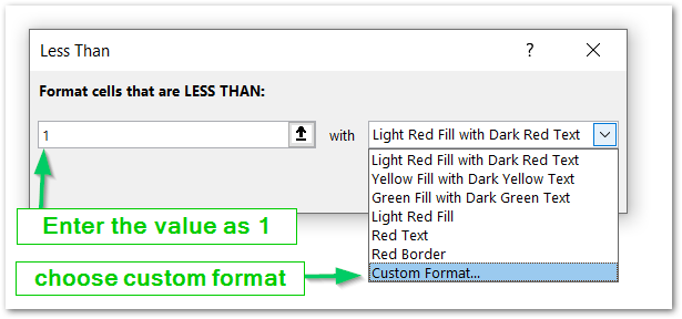
- Enter the value as 1 and choose the Custom formatting rule.
- Set the type field number format to ;;; ( three semicolons ) and click ok
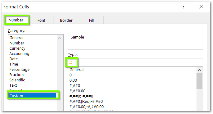
This would hide values less than 1 on the calendar.
- Add a new rule for the cell values greater than.
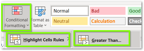
- Enter the following formula and then set the custom format to three semicolons to hide the invalid dates.
=DAY(EOMONTH($B$7,0))
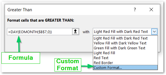
This would make the calendar start working logically.
We will now change the formatting.
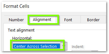
- Select the range B7:H7 and press the ctrl 1 keys.
- Go to the Alignment tab and set the horizontal alignment to Center Across Selection.
- Set the custom number format to dd mmmm
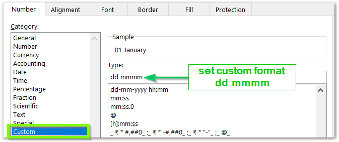
Thereafter, you can format the weekdays and headings as per your choice.
This brings us to the end.
