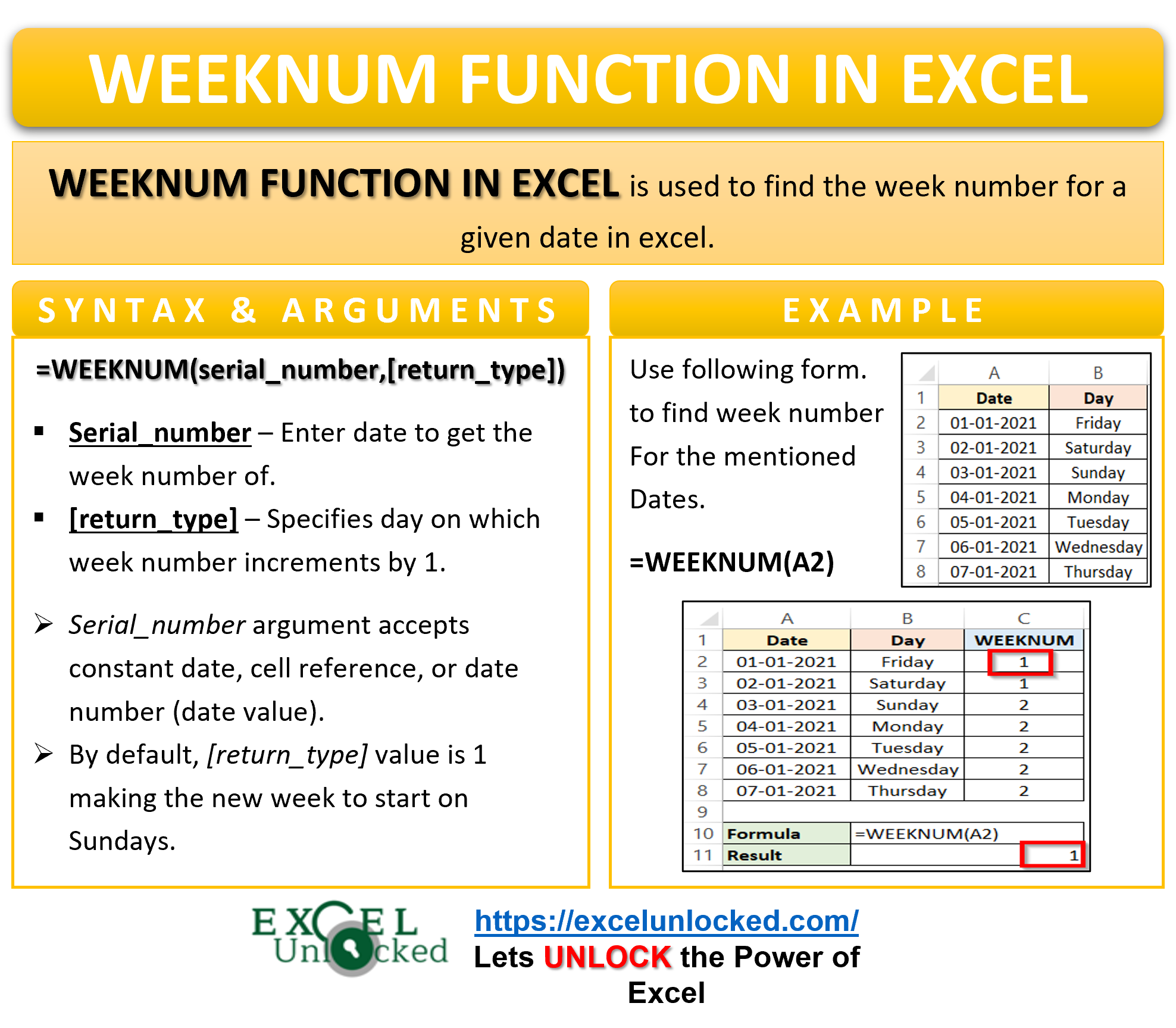
When we are working with dates in Excel, we might wish to know in which week of the year, this date falls. For example, what if I want to know in which week of the year my birthday comes?. This is going to be a very long calculation if I started counting the weeks from the beginning of the year. Thankfully, we don’t have to do it by ourselves when Excel has introduced the WEEKNUM Function.
In this tutorial we would learn how to calculate the week number of the date using the WEEKNUM formula in excel.
Here we go 😎
When to Use WEEKNUM Function of Excel
The word WEEKNUM represents “Week Number”. The function finds the number of the week on which a particular date falls. There are 365 days in a year (366 if leap year). When we divide 364 by 7 we get 52 complete years. The left 2 days might fall in the beginning or at the end of 52 complete weeks making the function to return the week number from 1 to 54.
The WEEKNUM formula forms part of the Date/Time Excel Function group.
Syntax and Arguments
=WEEKNUM(serial_number,[return_type])
The following points will explain to you, the function arguments of the WEEKNUM Formula.
- serial_number – This represents the date. It could be either a date in its actual format, numerical format or a cell reference.
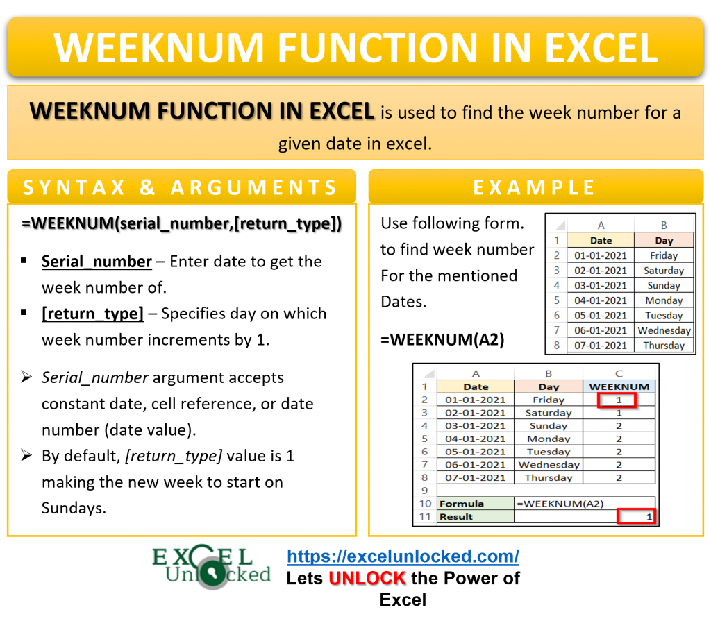
- return_type – This is an optional argument. It specifies the day on which the week number increments by 1. By default, its value is 1 making the new week to start on Sundays. Similarly when it is 2, the new week starts on Monday.
There are two systems to account for the first week of the year.
- System 1 – The week number 1 starts on first of January.
- System 2 – The first week will be the week containing the first Thursday of the year.
The following can be the valid inputs you can pass to the return_type function argument.
| Input value | New Week Starting on |
| 1 (default) | Sunday (System 1) |
| 2 | Monday (System 1) |
| 11 | Monday (System 1) |
| 12 | Tuesday (System 1) |
| 13 | Wednesday (System 1) |
| 14 | Thursday (System 1) |
| 15 | Friday (System 1) |
| 16 | Saturday (System 1) |
| 17 | Sunday (System 1) |
| 21 | Monday (System 2) |
Points to Keep In Mind About WEEKNUM Function
You should always keep the following points in mind before actually using the WEEKNUM Formula.
- Whenever the date is directly passed as serial_number, it must be enclosed within double quotation marks like this =WEEKNUM(“10-10-2021”).
- Valid excel dates have their numerical values. The dates start from 1-Jan-1900 as 1, 2-Jan-1900 as 2. The dates before 1 Jan 1900 when passed to WEEKNUM Function, makes it return a #VALUE! error message.
- We can also pass the numerical value of the date. For instance, the numerical value of date “10-10-2021” is 44479. The formula =WEEKNUM(44479) returns the same value as =WEEKNUM(“10-10-2021”) would. Learn more about excel date and time format in this link.
- When we do not pass any input to return_type function argument, the function automatically assumes it to be 1 and the new week starts on Sunday.
Examples to learn WEEKNUM Function of Excel
In this section of the blog, we will do some examples to learn the usage of the WEEKNUM formula.
Ex.1 – Basic Usage of WEEKNUM Function – Example
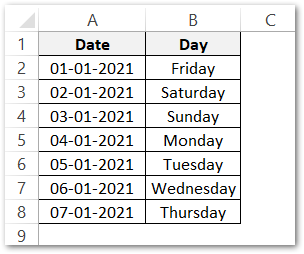
Let us say we have some dates from the starting of the year. Along with it, are the corresponding days of the month.
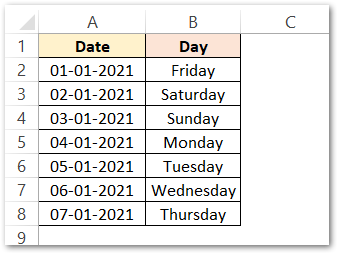
Use the following WEEKNUM Formula to get the results for the first date “01-01-2021”.
=WEEKNUM(A2)
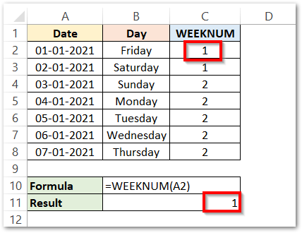
As a result, the formula returns 1. Use the Excel fill handle tool to copy the formula to the rest of the cells in column C.
Explanation – Cell A2 contains the date 1 Jan 2021. The date falls in the first week of the month, so the WEEKNUM formula returns 1. Similarly, the formula returns 1 for 2 Jan 2021.
On 3 Jan 2021, which comes on Sunday. The default value of the return_type function argument is 1. A new week starts here and the week number is incremented by 1. The second week starts on 3 Jan 2021 and thus the WEEKNUM formula returns 2 for it.
The rest of the dates also falls in the second week of the year, so the formula returns a 2 for them as well.
Also Read: WORKDAY.INTL Function in Excel
Ex.2 – Using Optional Argument ‘return_type’ – WEEKNUM Function
Let us see what happens to the week numbers of the above dates used in Example 1 when we pass different function arguments.
Use the following WEEKNUM formulas in cells C2, D2, E2, F2.
=WEEKNUM(A2,11)
=WEEKNUM(A2,12)
=WEEKNUM(A2,13)
=WEEKNUM(A2,14)
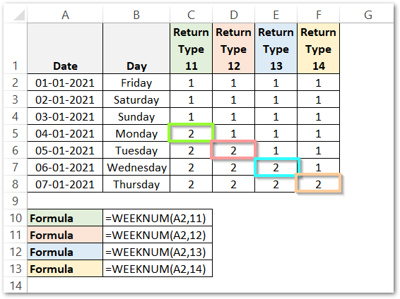
As a result, the formula returns the week number for 01-01-2021, but with different values of return_type argument.
Explanation – In the first formula, we have passed A2 as the date and 11 as the return_type function argument. As a result, the formula has returned the date 01-01-2021 to be in the 1st week of the year. When we copy the formula for the rest of the cells in column C, there comes a change in the week number for the date 04-01-2021. This is so because there is a Monday on that date and the week number is incremented by 1. So the formula returns 2 (C5) as the week number for the dates between 04-010-2021 and 08-01-2021.
Similarly, when we passed the return_type function argument to be 12, the new week starts on Tuesday. For the dates before 04-01-2021, the formula returns the week number for them to be 1. Once it comes a Tuesday on 04-01-2021 (D6), the formula starts a new week there and the date falls in the second week of the month.
The boxes indicate the days at which the week number is incremented by 1. For the return_type as 13 and 14, the day increments when there comes a Wednesday (E7) and Thursday (F8) respectively.
Ex.3 – Counting the Sales using SUMIFS and WEKNUM formula
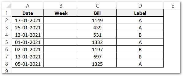
Let us now go a bit advanced. We have the order details of a company, as per the table below. We want to know the week at which each of the orders was received. Below are the order details.
Use the following WEEKNUM formula to get the week number of each of the dates.
=WEEKNUM(A2)
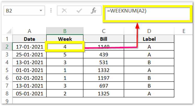
After we have got the week numbers for each of the dates, use this formula to get the total sales for different labels (A and B) in three weeks (1 to 3).
=SUMIFS(C2:C8,B2:B8,B10,D2:D8,A12)
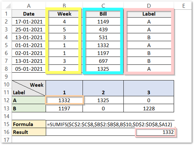
As a result, the WEEKNUM function of Excel has returned 1332 to be the sales of the first week for label A.
Explanation – The SUMIFS formula is used to get the sum of the range with the criteria specified.
We have set the sum_range to C2:C8 (Bills). The Criteria_range1 is B2:B8, with the criteria1 set to cell B10. So the function will filter out the records that correspond to “1” as the week. The second criteria A12 applies to the range D2:D8. The records that correspond to Label “A” as the Label will be considered. The function uses AND logic and finds the sum of Bills that have both Week 1 and the Label as A.
The formula when copied to the other cells, returns incorrect values because of Relative referencing that Excel uses while copying the formula.
Fixing the Cell Reference ( Absolute and Mixed Cell Referencing )
Whenever we copy a formula down in Excel, the cell references also move down by one cell. In this SUMIFS formula, we do not want the sum_range, criteria_range1, and criteria_range2 to change when the formula is copied for the cells B13, C12, C13, D12, D13. This is why we have locked these cell referencing by putting a $ for the range $C$2:$C$8, $B$2:$B$8, $D$2:$D$8. We have fixed both the Row numbers and Column Names to fix the complete Cell. This is known as absolute referencing.
For the formula, we have fixed criteria1 and criteria 2 by using mixed referencing. In Mixed referencing, we fix either the column ( the row number shifts to next ) or Row ( the column switches to next) while copying the formula. The criteria1 is set to B$10. The column will to C change when the formula is copied to cell whereas the row remains 10. The criteria1 will change to C$10 when copied to cell C12. Then D$10.
Similarly, for criteria 2, the referencing is $A12. The column is Fixed while the row shifts to next when the formula is copied down. It changes to $A13.
Thus, this should be the actual formula to get the results without errors.
=SUMIFS($C$2:$C$8,$B$2:$B$8,B$10,$D$2:$D$8,$A12)
This brings us to the end of the WEEKNUM Formula of Excel.
Thank you for reading 😉

