ACCRINTM Function of Excel – Calculating Accrued Interest

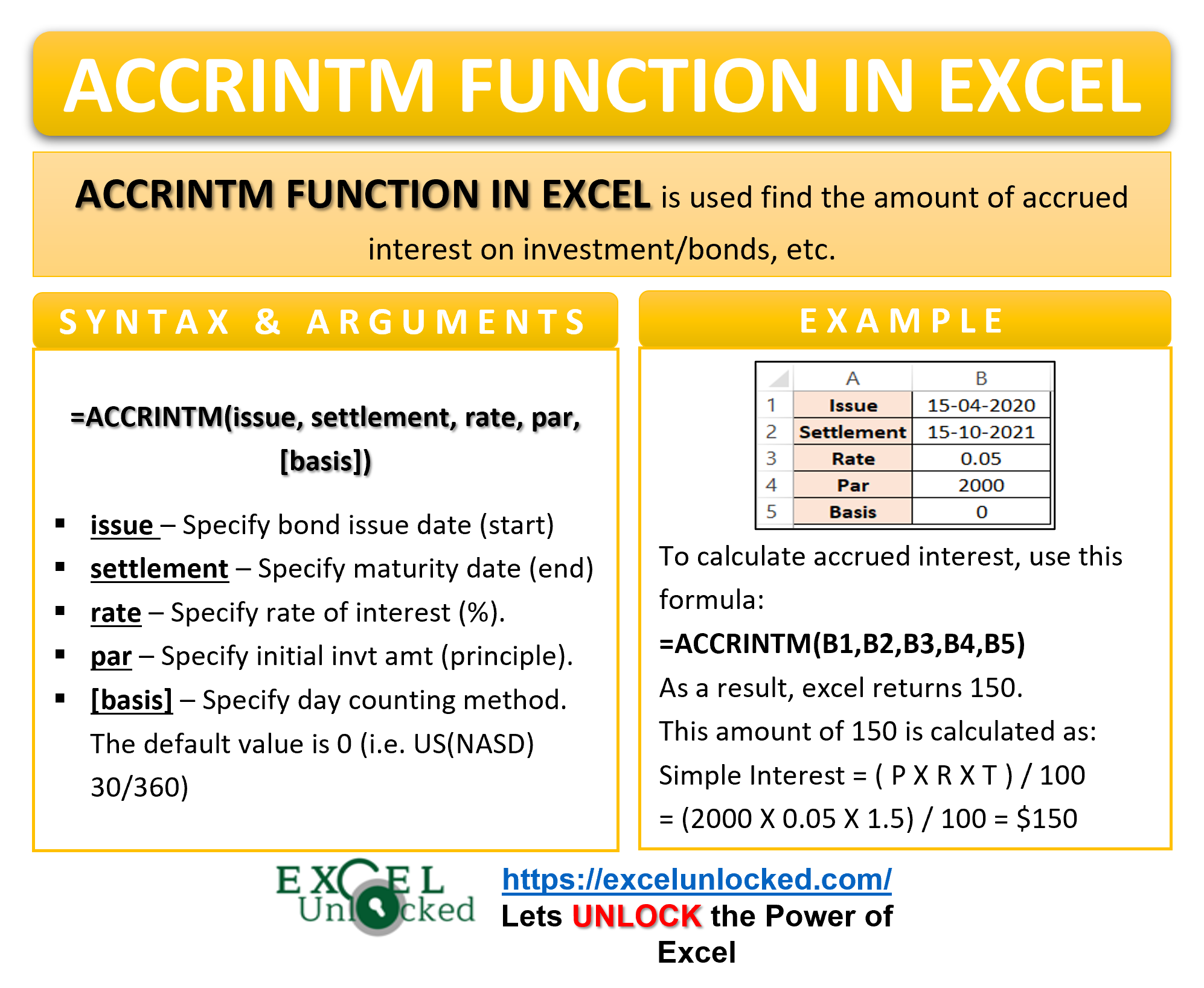
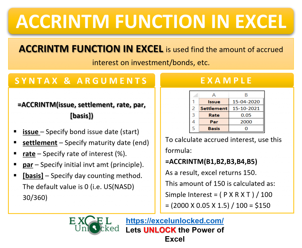
Have you ever heard about the term “Zero-Coupon Bonds”?. Well, a zero-coupon bond does not provide you the interest money in payments, instead returns the entire interests with the principal amount once the bond matures (expires). This is known as accrued interest (paid all at once at the end). This is when the ACCRINTM Function of excel comes into its usage.

In this tutorial, we would learn using the ACCRINTM formula in excel with examples.

Here we go 😎

When to Use ACCRINTM Function of Excel

The word ACCRINTM represents “Accrued Interest at Maturity”. The ACCRINTM formula in excel is used to find and calculate the accrued interest amount.

Maturity means the point at which the bond expires. There are securities that pay interests periodically or all at once. The ACCRINTM function returns the total amount of interest that the broker or a company pays on the face value of a bond, once the bond expires.

The function is categorized under the Financial functions of Excel.

Syntax and Arguments

=ACCRINTM(issue,settlement,rate,par,[basis])

The following points explain the required function arguments for the ACCRINTM formula of Excel.

• issue – This argument represents the date at which the security or a bond was issued.

• settlement – The argument refers to the expiry date of the bond.

• rate – It represents the annual coupon rate at which the interest amount is paid at the end.

• par – This is the face value of the bond or principal.

• [basis] – In this optional argument enter the day counting method for calculating the interest. It can have the following values.

Basis	Day Count
0 (default)	US(NASD) 30/360
1	Actual/Actual
2	Actual/360
3	Actual/365
4	European 30/360

To read more about these day count methods click here.

Points to Remember About ACCRINTM Formula

The following points must be kept in mind in order to actually use the ACCRINTM Formula.

• When no par value is specified, the formula considers it to be $1000.

• The function considers the default value of the basis to be 0.

• The function returns a #NUM! error if the issue and settlement dates are not in the right date format.

• The issue date cannot be greater then than the settlement date. For instace, the formula =ACCRINTM(Date(2021,1,1),DATE(2020,1,1),0.01,1000) will return a #NUM! error.

• The rate is not the interest percentage. It is the ratio of total annual interest paid to the face of the bond.

Examples to Learn Usage of Excel ACCRINTM formula

In this section of the blog, we will perform some practical examples to learn the usage of the ACCRINTM formula of Excel.

Ex. 1 – Simplest Example for ACCRINTM Function

In this example, let us say we have the values of the issue date, settlement date, annual coupon rate, and principle as follows.

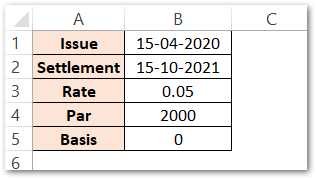
The value of the [basis] argument is taken as the default value (viz. 0). Use the following formula to get the accrued interest at the end of the settlement date.

=ACCRINTM(B1,B2,B3,B4,B5)

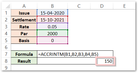
As a result, the excel ACCRINTM function returns the accrued interest amount as 150.

Explanation – Firstly, the function calculates the difference between the settlement date and the issue date argument to get the duration of the bond. In this example, the settlement date and issue date have a difference of 1.5 years. The annual interest rate is 0.05, or we can say 5% and the principal amount is $1000. Finally, the formula calculates the accrued interest amount using this calculation:

Simple Interest = P*R*T/100 (where P=2000, R=5%, T=1.5 years)

This gives the result of the formula to be 150.

Using TEXT function to format the results

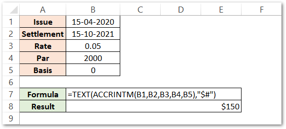
If you want to add a dollar sign ($) or any other text to the interest amount, use the below TEXT formula.

=TEXT(ACCRINTM(B1,B2,B3,B4,B5),"$#")

Ex. 2 – Using DATE Function With ACCRINTM Function

Many times while working with dates in excel, we might find out that the dates are not in the correct format. In such a scenario, we can use the DATE function for the issue date and settlement date in the ACCRINTM function in excel.

Let’s take this example – The bond was issued on 10-10-2021 and the settlement date is 10-10-2022. The annual coupon rate is 0.15 with a bond value to be $2550.

Use the following excel ACCRINTM formula to get the required results.

=TEXT(ACCRINTM(DATE(2021,10,10),DATE(2022,10,10),0.15,2550),"$#.00")

As a result, the formula returns $382.50

Explanation – The ACCRINTM function finds the accrued interest and then the TEXT function formats the result to the currency format. The DATE function returns the serial number for issue and settlement dates. The function finds the difference of dates 10-10-2022 and 10-10-2021 as one complete year. After that, the rate is 0.15 or 15% on a principal of 2550.

We can use this formula to verify the value of the ACCRINTM formula result:-

Simple Interest = P*R*T/100 (where, P=2550, R=15*1/100, and T=1 year)

The result comes out to be 382.5.

Moreover, the TEXT formula formats the accrued interest amount and adds dollar sign.

Evaluating the Formula Result

To evaluate the formula, follow these steps:-

• Select the cell containing the formula result (B2).

• Go to Formula Tab.

• In the Formula Auditing group, click on “Evaluate Formula” Button.

• The Evaluate Formula Dialog Box opens. Now Click on “Evaluate” button at the bottom to check the formula evaluation in steps.

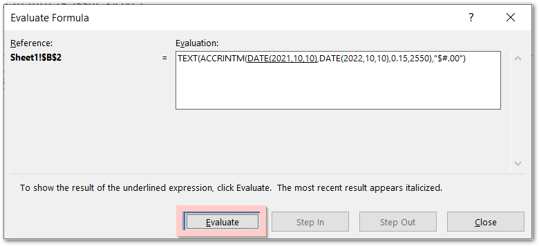
The following are the steps involved in formula evaluation.

• In the first click, the DATE Function returns the serial number for the Issued date as 44479.

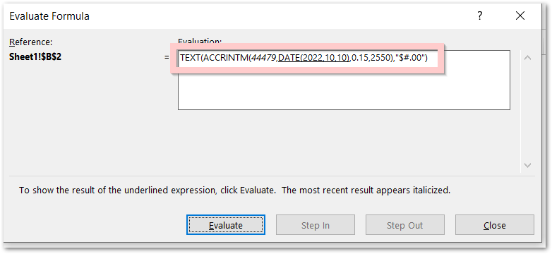
• On second click, the second DATE Formula returns the serial number for the settlement argument.

• On third click, gives the result of ACCRINTM Function to be 382.5

• At last, the final click on evaluate button gives us the value of accrued interest in currency format with two decimal places.

This brings us to the end of the ACRINTM Function Blog.

Thank you for reading;-)