When working with finances, we might feel the need to know the future value of a business investment after a certain period of time having a constant rate of interest. When saving money in a bank’s savings account that provides a constant rate of interest, we feel the need to know what would be the future value of my savings after 10 years from now. We can calculate it by adding interest after each accounting period to the savings, but this would be a long calculation. Excel provides us with the FV function to save us from the trouble!
When to Use FV Function of Excel
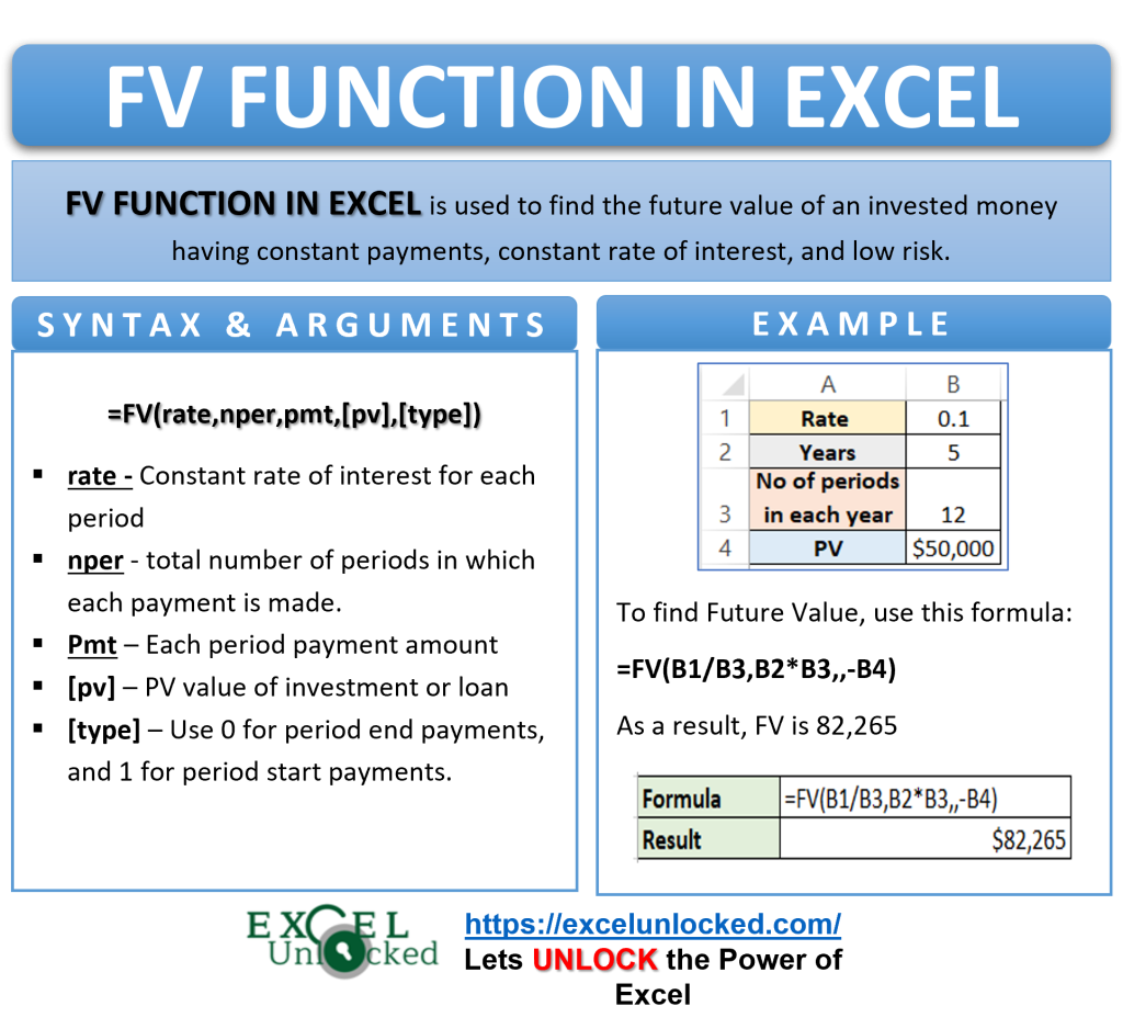
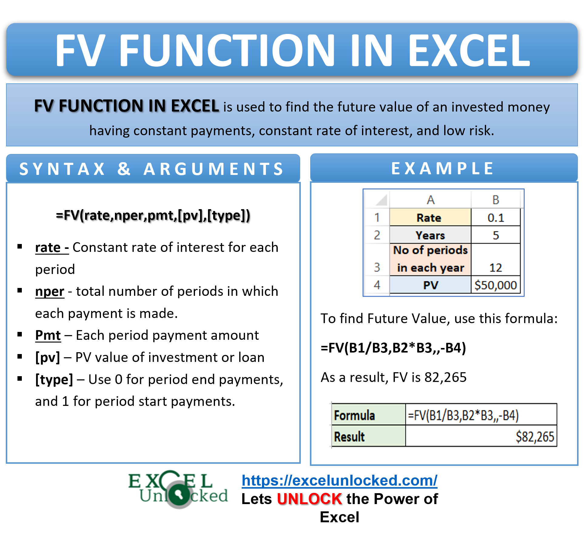
The word FV represents “Future Value”. The FV function is useful to get the future value of an invested money having constant payments, constant rate of interest, and low risk.
The FV function is categorized under the Financial Functions of Excel.
Syntax and Arguments
=FV(rate,nper,pmt,[pv],[type])
The following points will explain to you the FV function arguments.
- rate – This is the constant rate of interest for each period.
- nper – The argument represents the total number of periods in which each payment is made.
- pmt – It is the amount of payment you make in each period. If we omit this argument, then PV becomes a mandatory function argument.
- [pv] – This is an optional argument. pv specifies the present value of an investment or loan. It can be the principal value at the beginning.
- [type] – Type is 0 for payment done by the end of period and 1 if payment is completed at the beginning of each period. It is an optional function argument.
Points to Remember About FV Function
We should always keep these points in mind before using the FV formula.
- The default value of type is 0. In other words, if you didn’t specify this argument, the function will assumen that the payments are made at the end of the period.
- Although the pmt is not an optional argument, if we have specified pv then not specifying pmt would not return any error.
- pv and pmt are negative when the cash is going out of the business. For example, saving your money in bank is an outflow of cash. You make regular payments to get it saved in the bank.
- Simple interest is no longer a useful method. The FV Function of Excel uses Compound interest to calculate interest on the interest money+principal.
- Correct format to represent a rate of 15 percent is either 15% or 0.15.
Examples to Learn FV Function of Excel
In this section of the blog, we will learn some practical examples to learn the applications of the FV function.
Simplest Examples for Excel FV Formula
In this example, let us say there is a business that invested money of $50,000 at a constant annual interest rate of 10%. The company wants to know what will be the future value of this investment after 5 years from now. Below is the data:-

Consequently, cell B2 contains the total number of years and B3 has the total number of compounding periods for each year.
Use this formula to get the future value of this investment after five years.
=FV(B1/B3,B2*B3,,-B4)

As a result, the FV formula returns the future value of this investment to be $82,265.
Explanation – In the above formula, FV Function arguments have been specified as:-
- rate – This is the rate for each period. There is total of 12 periods in each year, so the annual rate (B1) when divides by number of periods of each year (B3) gives the interest for each period.
- nper – The total number of periods can be obtained by multiplying number of years (B2) by the number of periods in each year (B3).
- pmt – The business did not make any investment in payments in each period. The function argument will be ignored and function will assumen its value to be zero.
- pv – This is the present value of investment i.e -B4. It is negative because money is flowing out of the business.
- type – The default value is 0.
Looking behind the Scenes of FV Formula
The function will calculate the interest earned at the end of each period and then add it to the PV. When the next period comes, the compound interest will be calculated on pv+interest(earlier) and then added to PV.
Below is the future value of this investment at the end of one year. As mentioned, there are 12 periods each year.

In the first row, which is the initial value of the investment. After the first period, the interest earned is 417 (second row). The interest is added to the principal to give 50417 (50000+417). Now the new principal becomes 50417. On calculating interest of 0.1/12 gives 420 (third row). The interest when added to the principal gives 50837 (50417+420). The same procedure repeats for 12 periods give the future value of the investment at the end of one year to be 55236.
Similarly, the FV function has repeated this procedure for 12*5=60 periods to get the future value of the investment at the end of five years to be $82,265.

Calculating Future Value of Savings after 2 Years using FV Function
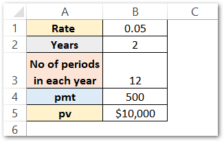
In this example, let us say we are saving money for purchasing a car. There is a balance of $10,000 already in the bank savings account. We can add to this saved amount by adding $500 each month to the savings. Below is the data:-

Bank gives an annual interest of 5% for savings accounts. There are 12 periods in each year and a total of 2 years. The present value of savings is $10,000.
Use this FV Function of Excel to get the savings after 2 years.
=FV(B1/B3,B2*B3,-B4,-B5)

As a result, the function has returned $23,642.
Explanation – The below points explain the passed function arguments in the above formula:-
- rate – We can obtain the rate for each period by dividing the annual rate by total number of periods in each year. In other words, rate is B1/B3.
- nper – We can get the total number of periods by multiplying number of periods by the total number of years. Consequently, it becomes B2*B3.
- pmt – This is the payment we are making at the end of each period (default value of type is 0). In this example it is -B4. IT is negative because of outflow of cash.
- pv – This is the principal amount we have already saved at the beginning i.e -$10,000 or -B5.
- type – The default value of type is zero. We will make payments of 500 at the end of each period.
The FV function will find the interest for each period i.e 0.05/12 on the PV and then add the pmt i.e 500 to the amount. Whenever the type is 0, there is no interest provided for that period on the pmt because it is deposited at the end of the period.
FV Formula Result Verification By Manual Method
We can verify the result of the above formula. Look at the data below.

PV is the account balance. Interest is the interest of 5/12 % earned on PV. PMT is the payment of 500 we are depositing at the end of the period. We have taken 12 periods in total to see the saved amount after 1 year.
Use the following formulas in Green, Red, Blue, and Yellow boxes respectively.
=B2*0.05/12
=B2+C2
=D2+E2
=F2

As a result, the function has returned 16,651 (F14) as the savings at the end of twelve periods (1 year)
We have used the Excel Fill Handle tool to copy the formula for the rest of the periods.
Explanation – We have calculated the interest of 5/12% on PV in cell C2 by the formula:- B2*0.05/12.
Cell D2 contains the principal amount added with the interest money on PV as =B2+C2.
After that, as the pmt paid at the end of each period is 500, adds to the account balance by using the formula =D2+E2.
The balance at the end of the first period becomes $10,541 in cell F2.
The balance at the end of the first period will act as the present value at the beginning of the second period. Thus the formula for PV of the second period is =F2.
Similarly, the procedure repeats for the twelve periods and the future value of the savings at the end of one year is $16,655.
Consequently, if we use the FV formula instead of the entire calculation to get the amount of savings at the end of on year, the formula is
=FV(0.05/12,12,-500,-10000)

You can see that the result is the same, but the FV formula saved us from the trouble!
Thank you for reading 🙂
RELATED POSTS
- NPER Function in Excel – Calculating Number of Periods
- NPV Function – How to Calculate NPV in Excel
- Excel XNPV Function – NPV With Irregular Cash Flows
- PMT PPMT IPMT Functions of Excel – Usage
- ISPMT Function of Excel – Interest Amount Keeping the Principal Constant
- IRR Function in Excel – Internal Rate of Return

