MONTH Function in Excel – Finding Month From Date

Sometimes, while working with dates in MS Excel, we might want to know the value of a month of a specific date. In that case, the MONTH function in excel has a very appreciable usage.

In this tutorial, we would learn how to use the MONTH Formula in excel with examples.

Here we go 😎

When to Use MONTH Function In Excel

The MONTH function in Excel is used to find the number value of the month of a specified date. For example, if we have the date as “1 January 2021” then the function will return the corresponding number of months as 1.

All the dates that land in January give 1, February give 2, March give 3, and so on. Therefore, the function returns a value between 1 and 12.

The Excel MONTH function is categorized under the date/time functions of Excel.

Syntax and Argument

=MONTH(serial_number)

The single argument of the MONTH formula in excel is the serial_number, explained below:

• serial_number – In this argument, specify a valid date in excel. The argument can accept a cell refrence, a date, numerical value of the date, or result of another formula.

Every valid date in Excel has its numerical value. The date value starts from 1, 2, 3 and so on, wherein 1 represents 1 January 1900, 2 represents 2 January 1900 as 2, and so on.

Therefore, any date earlier than 1 January 1900 is an invaid date.

Points To Remember About MONTH Function In excel

The following points must be kept in mind before the actual usage of the MONTH Formula of Excel.

• We can pass a date to the function in four ways:
  • Passing the actual date (within double quotes) like this “11-01-2021”
  • Using cell refrence like A2, B4, etc.
  • By using the result of some other function
  • Passing the numerical value of the date.

• MONTH function returns a #VALUE! error for the dates that do not exist. For example, 30-02-2021 or 32-5-1952. (see example 1)

• An invalid numerical value of the date to the MONTH function will return #NUM! error.

• The function cannot perform mathematical operations on the dates earlier than 1 january 1900. If you try to, then it will return #VALUE! excel error.

Examples To Learn The MONTH Formula of Excel

In this section, let us have a look at some of the practical examples to understand the usage of the Excel MONTH function.

Ex. 1 – Example | Using MONTH Function in Excel

In this example, let us learn the different methods of passing a date to the Excel MONTH formula.

The below image shows some dates in column A.

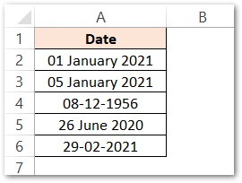
Suppose, we want to find the month number of the date in excel. To achieve this, simply use the following formula:

=MONTH(A2)

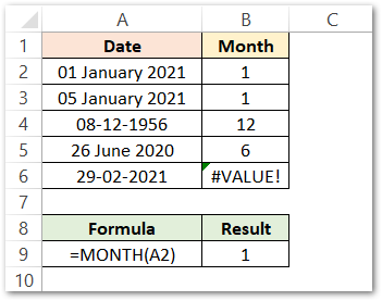
As a result, the formula returns 1.

Explanation – We have passed cell reference A2 as the serial_number argument. The function returns the corresponding value of the January month i.e. ‘1’.

Finally, copy and paste the formula to other cells in column A, or use the fill handle excel tool to copy the formula to cells below cell B2.

In Cell B6, the formula returns #VALUE! excel error because of the invalid date passed to the function argument.

Other methods to pass the date to the MONTH formula of excel includes the following:

=MONTH("10-10-2021")

=MONTH(44479)

=MONTH(DATE(2021,10,10))

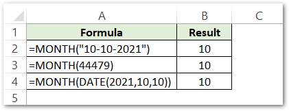
As a result, the formula returns 10.

Explanation – In the first formula, we have passed the exact date within double-quotes. Therefore, the function returns 10 as the number of month (October).

In the second formula, there is the numerical value of the date “10-10-2021” viz. 44479. The function returns the corresponding number of month as 10.

In the third formula, we have used the DATE function of Excel within the MONTH function.

With the DATE excel formula, you can construct a date having day, month, and year as input argument

Ex. 2 – Using Conditional Formatting with Excel MONTH Function

Let us suppose there is an online clothing business, and below are the details of its orders.

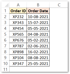
We want to highlight the orders that were received during August 2021.

Now, you need to follow these steps to apply conditional formatting using a formula in Excel.

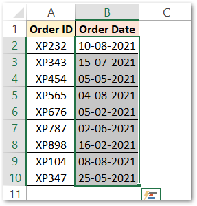
• Select the range of cells on which you want to apply the formatting.

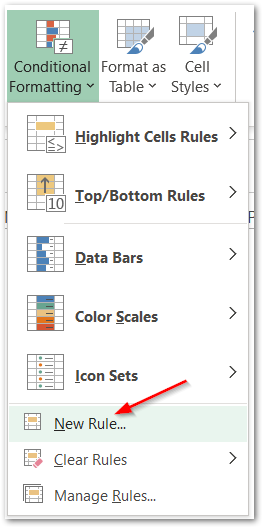
• Go to ‘Home’ tab. Under the ‘Styles’ group click on ‘Conditional Formatting’ button > ‘New Rule’ option.

• The ‘New Fomatting Rule. dialog box opens. Choose the option “Use a formula to determine which cells to format”.

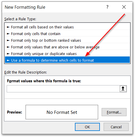
• We have used the IF Formula of Excel. Enter the following formula and click on the format option to set the format if the formula returns TRUE result.

=IF(MONTH(B2)=8,TRUE,FALSE)

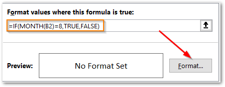
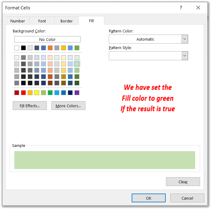
• In the format cells dialog box, go to the fill tab and select the color of your choice (like green) and click on OK.

As a result, this formula specified in ‘Conditional Formatting’ will highlight all the cells that contain the dates lying in the month of August.

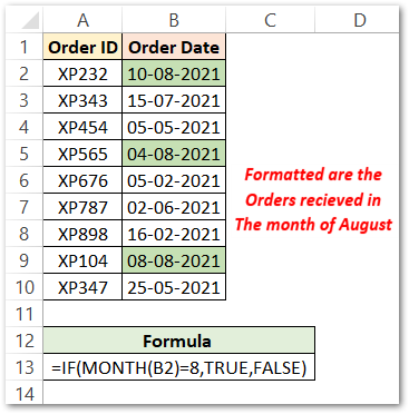
Explanation – We have entered the formula =IF(MONTH(B2)=8,TRUE,FALSE). This is an IF formula. The condition used here is MONTH(B2)=8. The entire formula reads like this – If the month value of the cell B2 is equal to 8, then return TRUE, else FALSE. If it returns TRUE, then the cells get formatted as green.

This brings us to the end of this tutorial on how to use the Excel MONTH function.

Thank you for reading 🙂