EOMONTH Function in Excel – Getting Last Day of Month

The EOMONTH function in excel has a very appreciable usage in performing an arithmetic operation on dates. In this tutorial, we would learn how to use the EOMONTH formula in excel, along with its usage, examples, and many more.

Here we go 😎

When to Use EOMONTH Function in Excel

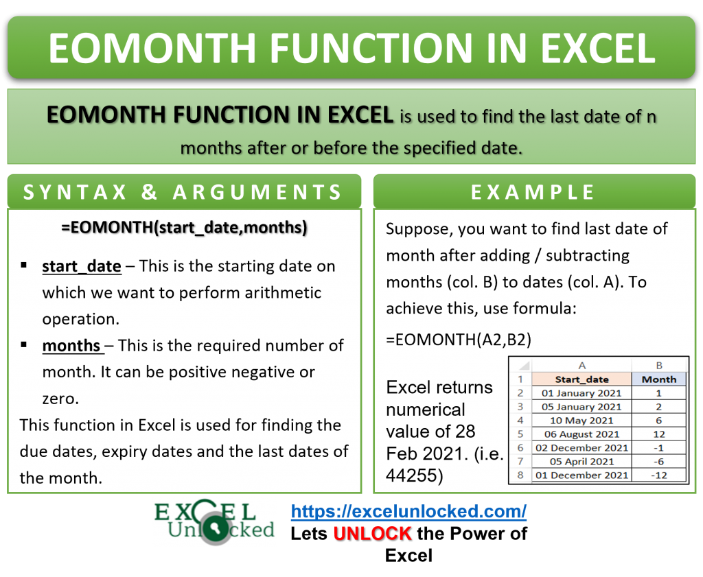
The word EOMONTH represents “End of the month”. The Excel EOMONTH function is used to find the ending date (i.e. last date) of a month before or after ‘n’ months from a specified date. The function belongs to the date/time functions of Excel.

This function comes into its use for finding the ending date of a month. Another practical example of this function includes finding the total sales up to the last date of this month using the EOMONTH formula along with the SUMIFS Formula of Excel.

Syntax and Arguments

=EOMONTH(start_date,months)

The below points explain the arguments of the EOMONTH Function of Excel.

• start_date – In this argument, specify the date on which you wish to add/subtract months and return last day of a month.

• months – This is the argument representing the number of months. Put a positive value of this argument if you want to move ahead in time and negative value if you want to move back in time.

The function returns the numerical value of the date. To get the date in the date format, simply change the cell format, as described in the section below.

Changing Cell Format in Excel

The Excel functions cannot perform any calculation on the actual dates. Therefore, it firstly converts the date into its numerical value.

Each date in excel has its own serial number starting from 1 Jan 2019 as 1, 2 Jan 2019 as 2, and so on.

EOMONTH Function of Excel will add or subtract the specified number of months to a date and return the last day of that month as its numerical value. The numerical value needs to be formatted to date to get the required result.

Below are the steps to change the numerical values into the date format.

• Select the range of cells that you wish to change the format of.

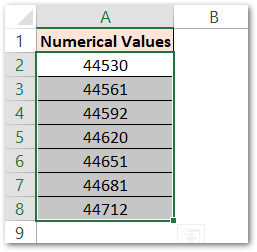
• To open the format cells dialog box, hit Ctrl + 1 on your keyboard.

• In the ‘Format Cells‘ dialog box that appears, select the desired date format under the ‘Date’ category, as shown below.

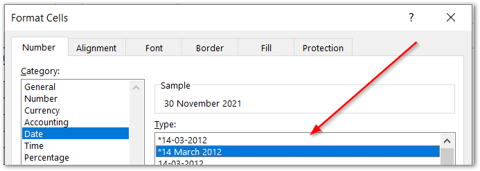
• As a result, the numerical values will now change into their corresponding dates as shown in the image below.

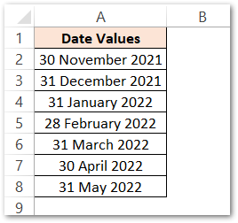
Learn more about excel date format in this blog – All About Excel Date Format.

Points to Remember | Excel EOMONTH Formula

The following points must be kept in mind before the actual usage of the EOMONTH Function of Excel.

• The function does not return actual date, but its numerical value in Excel (see above section)

• The function will return a #VALUE! error for the invalid dates like 32 Jan 2021 or 29 Feb 2019.

• We can also pass the numerical value of date to the start_date function argument. In case the value entered is invalid then the function returns a #NUM! error.

• The numerical values of dates start from 1 Jan 1900 as 1. The function cannot perform arithmetic operation on dates earlier than 1 Jan 1900. It will give a #VALUE! error in excel.

• The function can be used to find the starting date of a month.

Examples to Learn the Usage of EOMONTH Formula of Excel

In this section of the blog, let us have a look at some practical examples to learn how does the EOMONTH function in Excel.

Ex. 1 – Learning Basics of EOMONTH Function via Example

The below example image shows dates and the value of corresponding months.

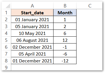
Suppose, you want to find the last date of the month after adding/subtracting the particular number of months (column B) to dates in column A.

To achieve this, simply use the following formula in cell C2.

=EOMONTH(A2,B2)

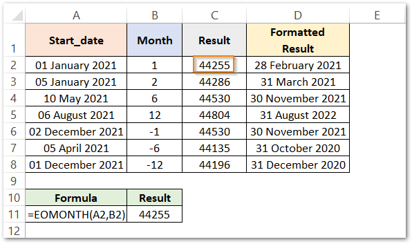
As a result, the formula has returned 44255.

Explanation – We have passed the start_date as A2 and the months as B2. The function returns the numerical value (44255). The value 44255 represents the last day of the month after adding one entire month to the start_date.

Once we have obtained the numerical value, it can be converted into date format as explained above section. Consequently, the final result of the formatted cell is “28 February 2021” (last day of the month after adding one month to the “1 January 2021”).

The formula can be very easily copied to the rest of the records by double-clicking on the bottom right corner of cell C2 (using fill handle excel tool).

In cell B6, the month argument is a negative value. As a result, the function goes backward and return the last day of the month by subtracting one month from 02 December 2021.

Ex. 2 – Finding Total Number of Orders From the Beginning To The End Of Month

The below example image contains order details in a bakery shop.

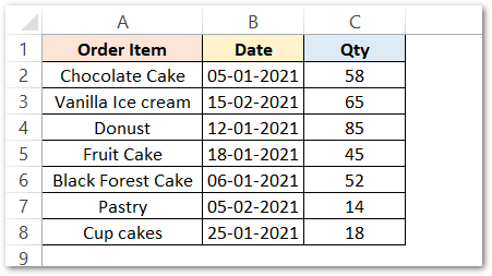
Now, the bakery owner wants to determine what is the total number of orders received in the month of January (i.e. between 1 Jan 2021 and 31 Jan 2021).

Use the following formula to get the desired results.

=COUNTIFS(B2:B8,">="&EOMONTH(B2,-1)+1,B2:B8,"<="&EOMONTH(B2,0))

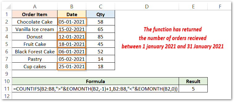
As a result, the formula returns 5.

Explanation:

To count the number of values between two dates in excel, we have taken the help of the COUNTIFS excel function. Criteria_range remains the same (B2:B8) for both the criterion. The first criteria is “>”&EOMONTH(B2-1)+1 which returns the first date of the month. In this expression, EOMONTH(B2-1) finds the serial number for “31 December 2020” and +1 adds 1 to the serial number. Hence final value is “1 January 2021”.

The second condition “<“&EOMONTH(B2,0) returns the last date of the same month i.e. “31 January 2021”.

Finally, the COUNTIFS formula counts the number of orders between these two dates.

Thank you for reading 🙂