What is Excel Conditional Formatting?

Conditional Formatting is a very fascinating topic in excel. It might seem confusing to some people but is one of the straightforward things to learn. So let us begin learning.

What is Conditional Formatting?

Conditional Formatting means that the cells are formatted based on some condition. The cell would be formatted only if the cell content satisfies the condition. The cell format could be fill color, font color, cell border, or style.

Whenever, the cell content changes, the conditional formatting automatically updates itself as per new cell data. It is dynamic and flexible. Any change in the cell data is automatically reflected.

We can apply conditional formatting on a range of cells, rows, or columns. The cell format can be preset like color scales, Data Bars, and Icon Sets or we can define our formats.

You can have the practice workbook to follow along.

Where to Find Conditional Formatting Option?

To apply conditional formatting:-

• Select the range of cells on which you want to apply the formatting.
• Follow the path Home Tab > Styles Group > Conditional Formatting

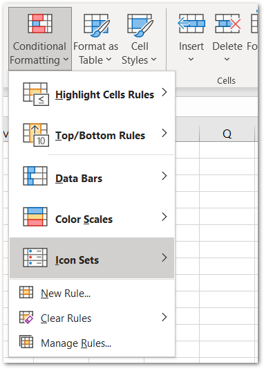
From here, you can apply all types of conditioned – formatting.

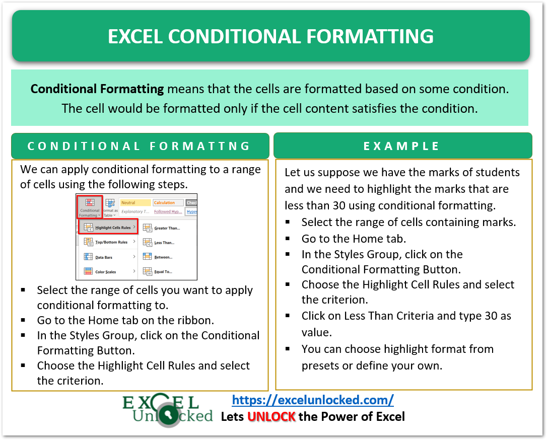
Ex 1 – Highlighting Values using Criteria Greater Than

Let us say we have got the debate scores of different participants. The scores are assigned out of 100.

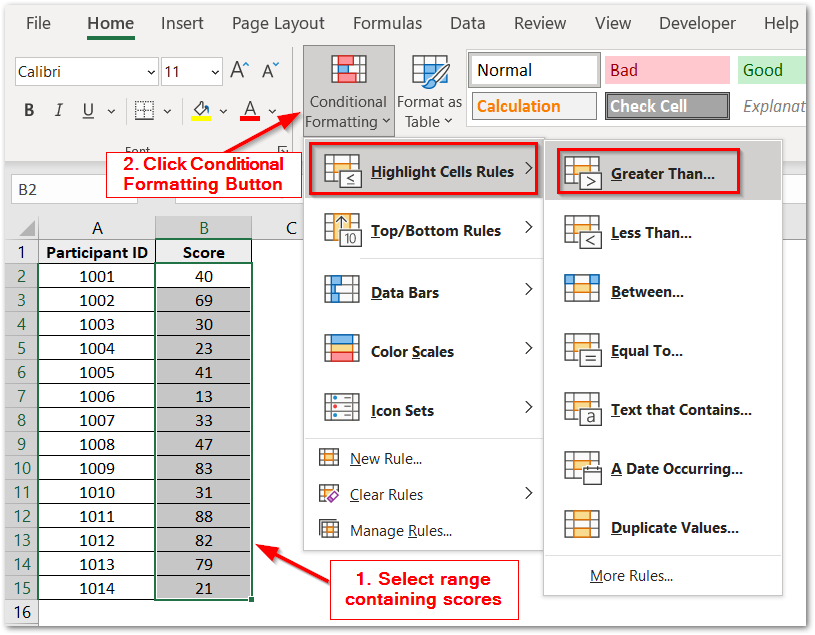
• Select the range of cells containing scores of students.
• Click on the Conditional Formatting button in the Home Tab.
• Click on Highlight Cell Rules from the drop-down menu and choose Greater Than Criteria.

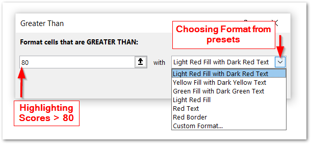
• Set the value as 80 because we want to highlight the scores that are greater than 80. Thereafter you can choose the format for highlighting the cells from the presets. We are choosing Yellow Fill with Dark Yellow Text.

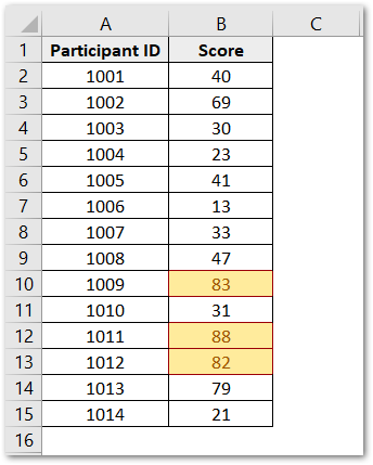
Note that if we change any score, it would be automatically highlighted if the new score is > 80.

Ex 2 – Highlighting the Values using Less Than Criteria

Let us say we need to highlight the marks of students who scored less than 30 marks in a class test out of 100 marks.

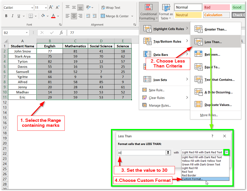
• Select the range of cells containing the marks of students.
• Click on the Conditional Formatting Button. In the highlight cell rules, choose Less Than Criteria.
• Set the value to 30 so that marks less than 30 are highlighted.
• Instead of picking the highlighting format, we would now set the custom format for highlighting the marks < 30

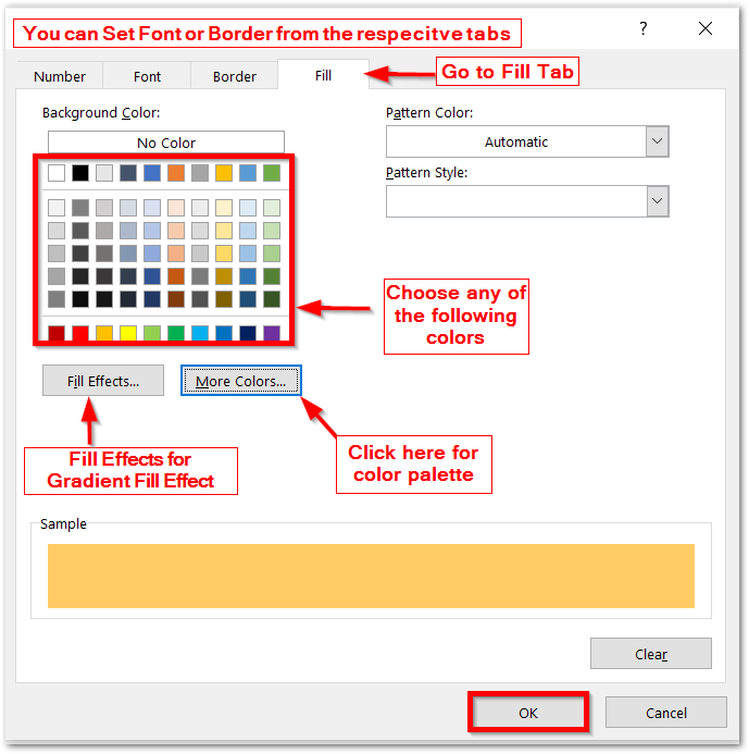
• This would open the Format Cells Dialog Box. From the fill tab, choose the fill color from the Given Colors or the Color Palette. You can also set the Font style and border for the highlighted cells. Click OK.

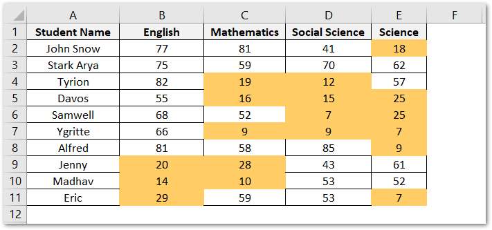
So you can see that the marks less than 30 are highlighted with the custom formatting we applied.

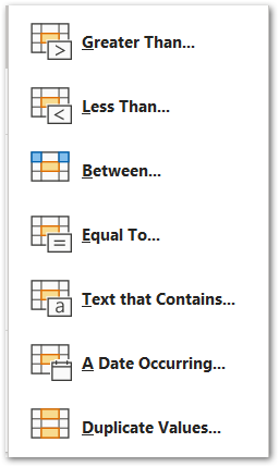
In a similar way, we can apply formatting using another criterion like:-

• Between
• Equal To
• Text that Contains
• A Date Occurring
• Duplicate Values

This brings us to an end.

Thank you for reading.