Data Bars in Excel – Add and Customize

Previously we have learned the basics of conditional formatting. Today we would learn an important part of conditional formatting. Data Bars in Excel are very helpful to make your data more readable and easy to analyze at a glance.

So let us begin learning.

What are Data Bars?

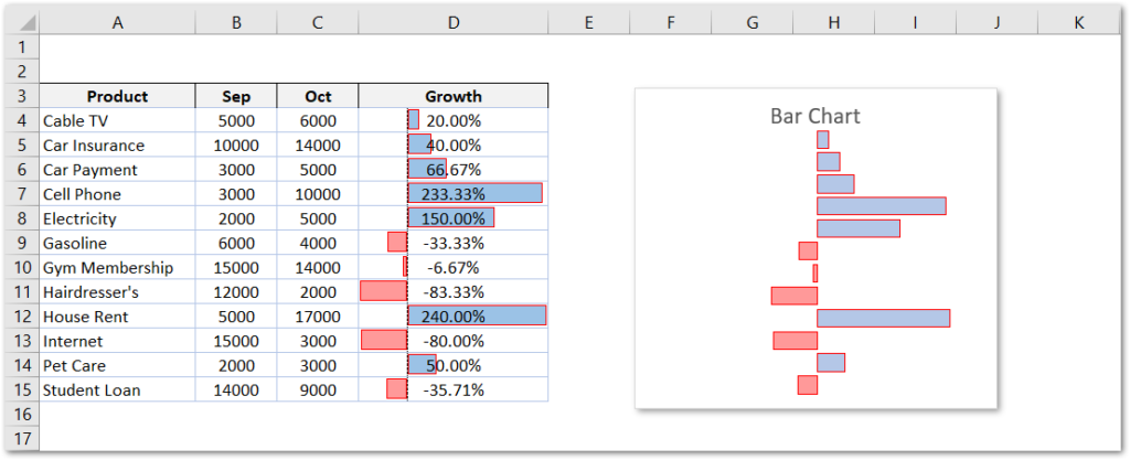
Data bars are horizontal bars in the cells of the spreadsheet whose length helps us to compare different cell values. The longest bar indicates a maximum value while the shortest bar indicates the smallest value. It is different from a normal bar chart as a bar chart is a whole object while Data Bars are contained in the cells.

You can grab a practice workbook to practice along with us while reading.

How to Add Data Bars?

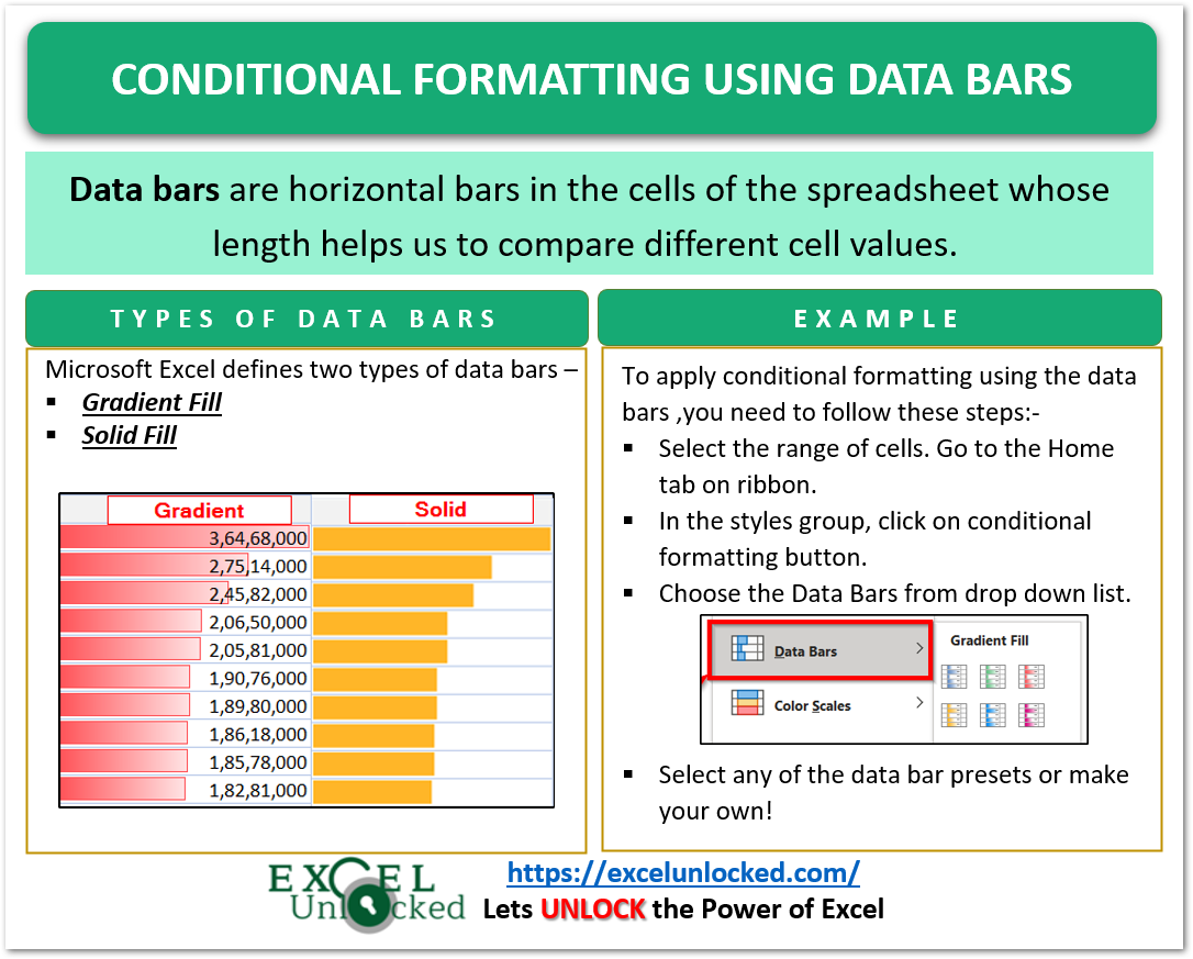
There are mainly two types of data bars in excel based on the fill color:-

• Gradient Fill – Used more frequently.
• Solid Fill – Used when the cell only contains data bars and the cell value is hidden.

To add data bars to a range of cells simply:-

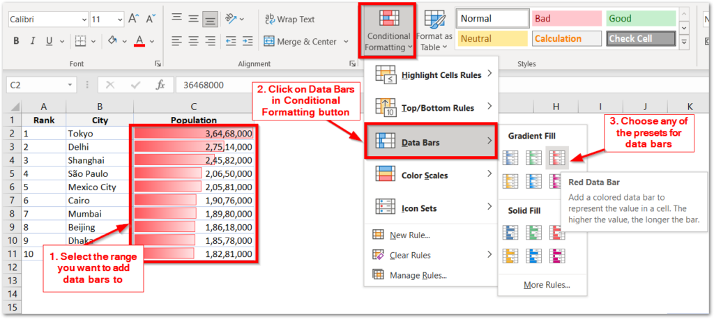
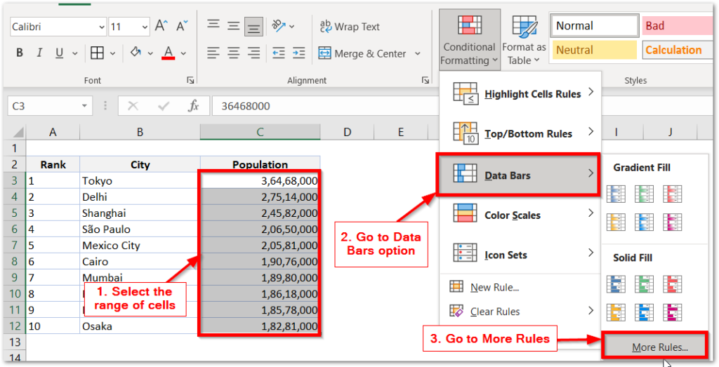
• Select the range of cells where you wish to add data bars.
• Click on the Conditional Formatting button in the Home tab under the Styles Group.
• Choose Data Bars and select a data bar from the provided Gradient and Solid Fill Presets.

• You can also choose from any of the Solid Presets for Data Bars. Just hide the cell contents for that range because solid data bars make the text inside the cells harder to read and we should hide the values instead.

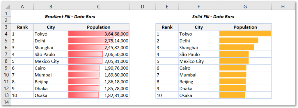
To hide the cell contents, select the range of cells and press Ctrl 1 key. Set the Custom Number format and in the type field, enter ;;; three semicolons.

How to Customize Data Bars?

There are several Gradient as well as Solid Fill Presets for Data Bars. When none of them fits our needs, we can make custom data bars as explained below.

• If you have to add new data bars, then go to the Data Bars option in the Conditional Formatting button in the Home tab and click on the More Rules button
• If you have existing data bars and you need to customize them, then select the range of cells and press the Alt O D key. Find the Data bar rule on the list and click on the Edit Rule option.

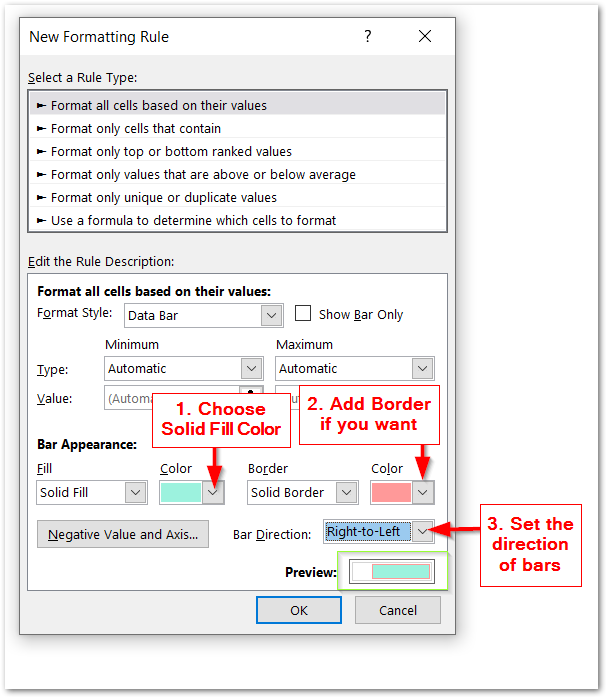
• This opens the New Formatting Rule/Edit Formatting Rule Dialog box. Select the fill color, the border color ( optional ), and the direction of the bars.

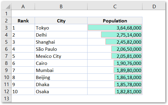
As a result, we have got the customized data bars as follows.

This brings us to an end.

Thank you for reading