Today, we are going to learn a very interesting topic. Conditional Formatting is used to format the cells based on some condition. Color Scales are one of the methods using which we can apply conditional formatting to our data set.
So let us begin learning.
What is Color Scale?
Color Scale colors the cells based on the magnitude of the value it contains. We can apply conditional formatting using these color scales.
Grab the practice workbook from here.
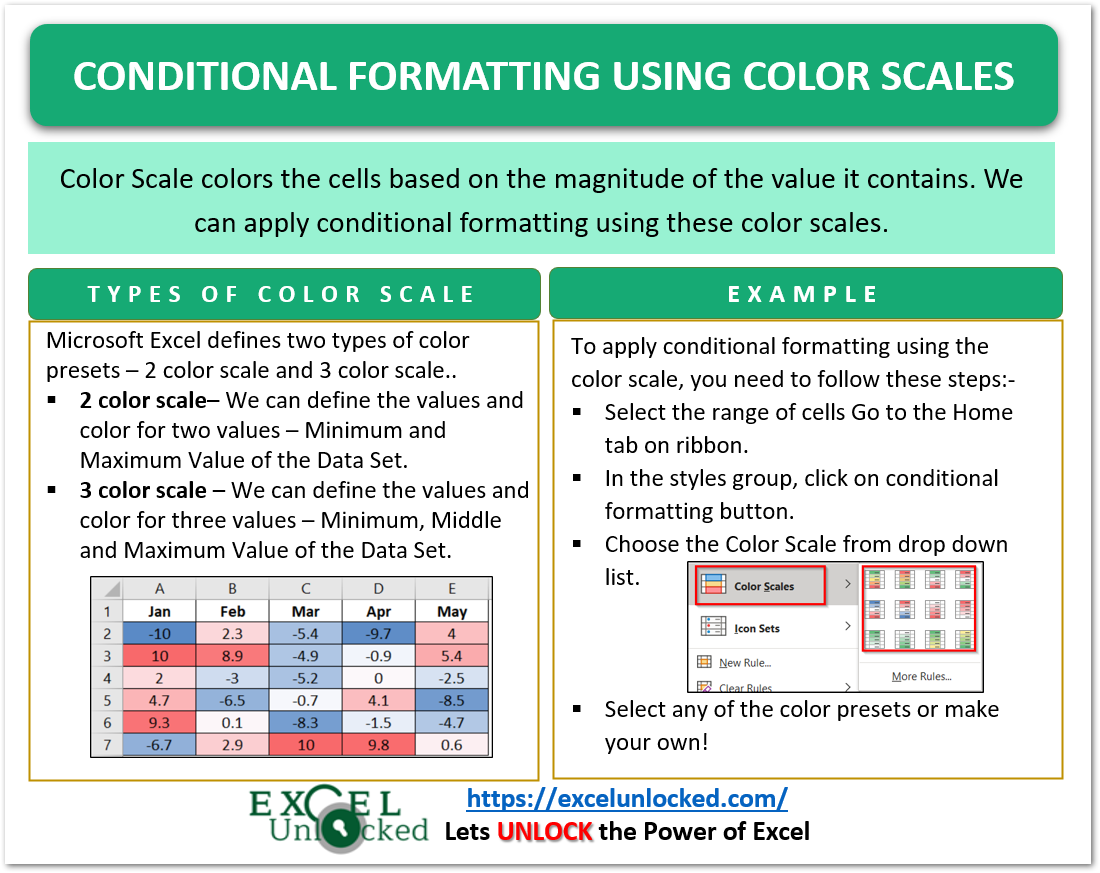
Microsoft Excel defines two types of color presets – 2 color scale and 3 color scale.
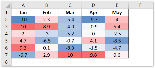
This is a 3-color scale ( Min, Max, and Mid ) where the maximum value is 10 (A3). It is highlighted with dark red while the minimum value is -10 in cell A2 which is highlighted in Blue. The different shades of both colors indicate the value a cell contains. The values lying in the middle of the maximum and the minimum value are in white. There are values close to zero.
We can customize a color scale very easily.
How to Add a 2 Color Scale? – Conditional Formatting
let us suppose we have got the grades of different students as follows.
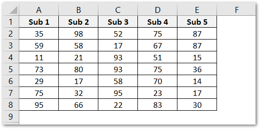
To highlight these cells based on the marks, we can use the two color scale. Implement the following steps.
- Select the range of cells A2:E8.
- Go to the Home tab on the ribbon. In the Styles Group, click on the Conditional Formatting Button.
- Choose the white red color scale.
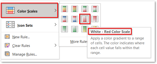
This would format the different subject marks such that the highest marks would be in white color and the lowest marks in red.
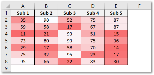
So you see, now we can easily figure out the marks that are result spoilers and are lowest or need improvement. Darker shades of red are highlighting the lower values.
How to Add 3 Color Scale?
3 color scale would contain three colors to highlight the cell contents. Let us suppose we have the percentage of monthly revenue for 5 years.
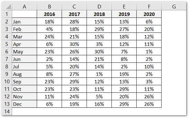
To add a 3 color scale, follow these steps:-
- Select the range of cells A2:F13
- Click on the Conditional Formatting button under the styles group in the home tab.
- Click on More Rules in the Color Scale Section. Note that you can either make your own rule for color scale regarding formats and min, mid and max values or you can just pick a 3-color preset.
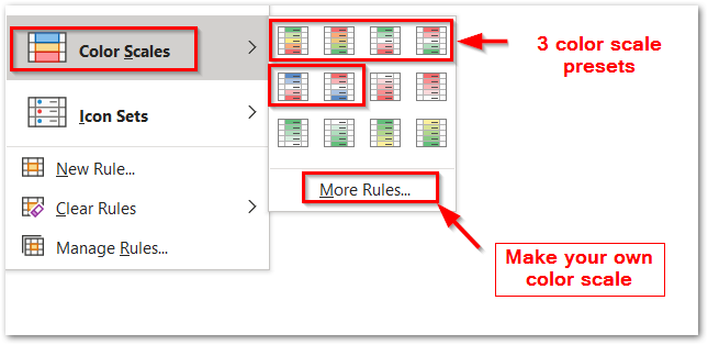
- This opens the New Formatting Rule Dialog box.
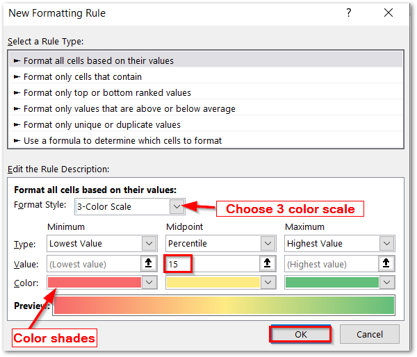
- Choose the 3 color scale in the Format Style Field. Change the Midpoint value to the 15 percentile as the percentage of revenue lies between 1 and 30 percent. Click OK.
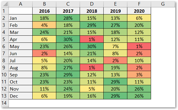
As a result, the lower values are in red, the middle values are in yellow, and the higher values are in green color.
This brings us to end. Thank you for reading.
