How to Count Duration in Hours Between Two Dates?

The Date and time in Excel are stored as decimal numbers. There are times when we need to calculate the total number of hours between two dates or times. There are many different approaches to count the duration in hours between two dates.

So let us begin learning.

Method 1 – Difference between two Dates in Hours

This is the first method to count the duration in hours between two dates. You can use this practice workbook to practice along with us.

Since the dates in Excel are stored as decimal numbers, we can simply find the difference between two dates and then multiply the result by the total number of hours in a day.

The total number of hours in a day is 24, the syntax to get the date difference in hours becomes:-

=(Date1-Date2)*24

Now, let us suppose we have the following starting and ending dates for a period of time.

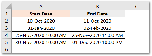
The 4th and 5th row contains dates along with time value. We can use the following formula in cell C2 and then copy it down for the range C2:C5.

=(B2-A2)*24

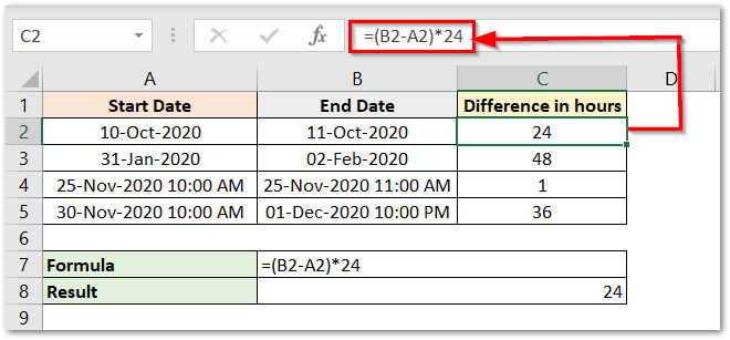
As a result, we have successfully got the difference between the End Date and the Start Date.

Explanation – We have taken the End Date in Column B and the Start Date of the period in Column A. We would take the difference between two dates indicated by A2-B2 and then multiply it by the total number of hours in a day:-24.

Method 2 – Using the TEXT Function

This is the second method to count the duration in hours between two dates.

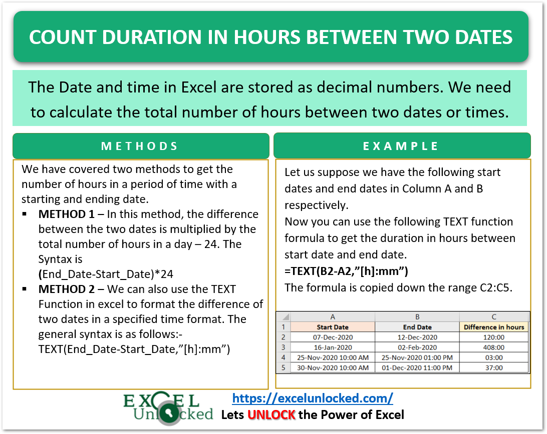
The TEXT Function converts the text into any specified number format. When the difference between the end date and the beginning date of a period is converted into a standard time format, we get the difference in hours between the two dates.

Therefore, the general syntax for this method is as follows.

=TEXT(End_Date-Start_Date,"Time_Format")

Here is the time format enclosed in double quotes. You can use any other time format like hh:mm, hh:mm:ss, or hh:mm AM/PM as per your requirement.

Now, let us implement the method with an example.

Use this TEXT Function formula in column C.

=TEXT(B2-A2,"hh:mm")

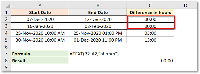
Here you can see that the formula works correctly when the difference between the two dates is less than 24 hours. For cells C2 and C3, the difference in dates is more than 24 hours, which is why we see 00:00 as if the start and end dates are identical and there is no time period between the two dates which is not true.

To resolve this issue, we need to update the time format to:-

=TEXT(B2-A2,"[h]:mm")

This formula would enable us to show the time values greater than 24 hours.

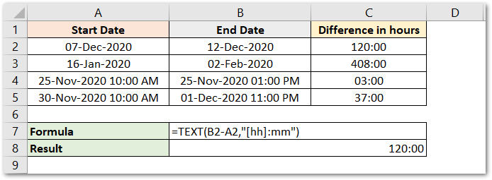
Now, you can see the exact number of hours between the four periods of the ending and starting dates.

This brings us to an end.

Thank you for reading.