XLOOKUP Function in Excel – Advanced Lookup

The excel XLOOKUP function is a newly introduced lookup formula/function in excel.

This function has many more advanced functionalities over the age-old lookup functions like INDEX/MATCH and VLOOKUP/HLOOKUP formula in excel.

In this tutorial, we would unlock this new excel lookup formula – XLOOKUP formula in excel, along with its syntax, argument, and simple examples.

Here we go !! 😎

I Do Not Have XLOOKUP Formula in My Excel …..

After introduction of the XLOOKUP excel formula, I this questions from many of my colleagues – “Hey! How to get access to XLOOKUP formula in Excel?”

See below points for its answer:

• Currently, Microsoft has released the XLOOKUP function only for the Office 365 excel users.

• However, currently, excel XLOOKUP formula is not available for older excel versions (Excel 2010, 2013, 2016, and 2019). The reason for this is still unknown.

• The XLOOKUP formula is supported by both the operating systems – MacOS and Windows.

• This function is also available in web version of excel (excel online).

XLOOKUP Formula Missing in My Office 365 ….

Sometimes, even though you are Excel Office 365 user, you do not have access to the XLOOKUP excel formula. In such a scenario, follow the undermentioned steps:

• Open excel workbook and navigate to File tab > Account option.

• In the ‘Product Information’ section, click on the option ‘Office Insider’ > ‘Join Office Insider’, as shown below:

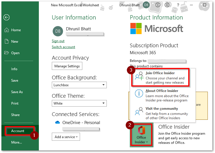
As a result, you would join the office insider program and finally get instant access to any new functions released by Microsoft 😉

What is XLOOKUP Function in Excel?

The new XLOOKUP excel function is an improved version of the old lookup functions like INDEX/MATCH and VLOOKUP/HLOOKUP formula in excel.

This new formula function does everything that the VLOOKUP and HLOOKUP formula do, with some added functionalities.

Using XLOOKUP function in excel, you can perform both vertical as well as horizontal lookup of value using this single formula. There is now no need of using separate formulas (VLOOKUP and HLOOKUP) for it.

The excel XLOOKUP function is useful to find and search for a particular text/value in a dataset and then return corresponding value from other excel row or column in the dataset. XLOOKUP can search both ways – horizontal and vertical.

Syntax and Arguments

=XLOOKUP(lookup_value, lookup_array, return_array, [if_not_found], [match_mode], [search_mode])

Below is the explanation of the XLOOKUP syntax and its six arguments:

• lookup_value – In this argument, specify the lookup value to search for.

• lookup_array – In this argument, specify the cell range or name range in which you want to search lookup_value.

• return_array – Here, specify the corresponding cell range or name range (row/column) from which you want to extract the value.

• [if_not_found] – (optional argument) Specify the text/value that you want to return, if the function does not find the lookup_value in lookup_array. Since it is an optional argument, the XLOOKUP function returns #N/A error if you keep this argument blank. (see example 2)

• [match_code] – In this argument, you specify 0, -1, 1, or 2 based on how you want excel to perform matching of values. (discussed in detail later – Example 4 & 5)

• [search_mode] – In this argument, you enter 1, -1, 2, or -2 to specify how should function search the value in lookup_array. (discussed in detail later – Example 6)

XLOOKUP Excel Function Examples

Finally, we have reached to a point when we can start understanding how XLOOKUP formula works in excel.

In this section, we would see some basic and interesting examples of XLOOKUP excel formula on following dataset about student’s marks.

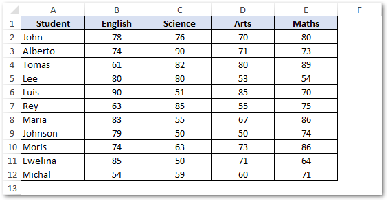
Use Download button below to get the sample practice file for XLOOKUP function.

Example # 1 – Fetch Value From Corresponding Row/Column

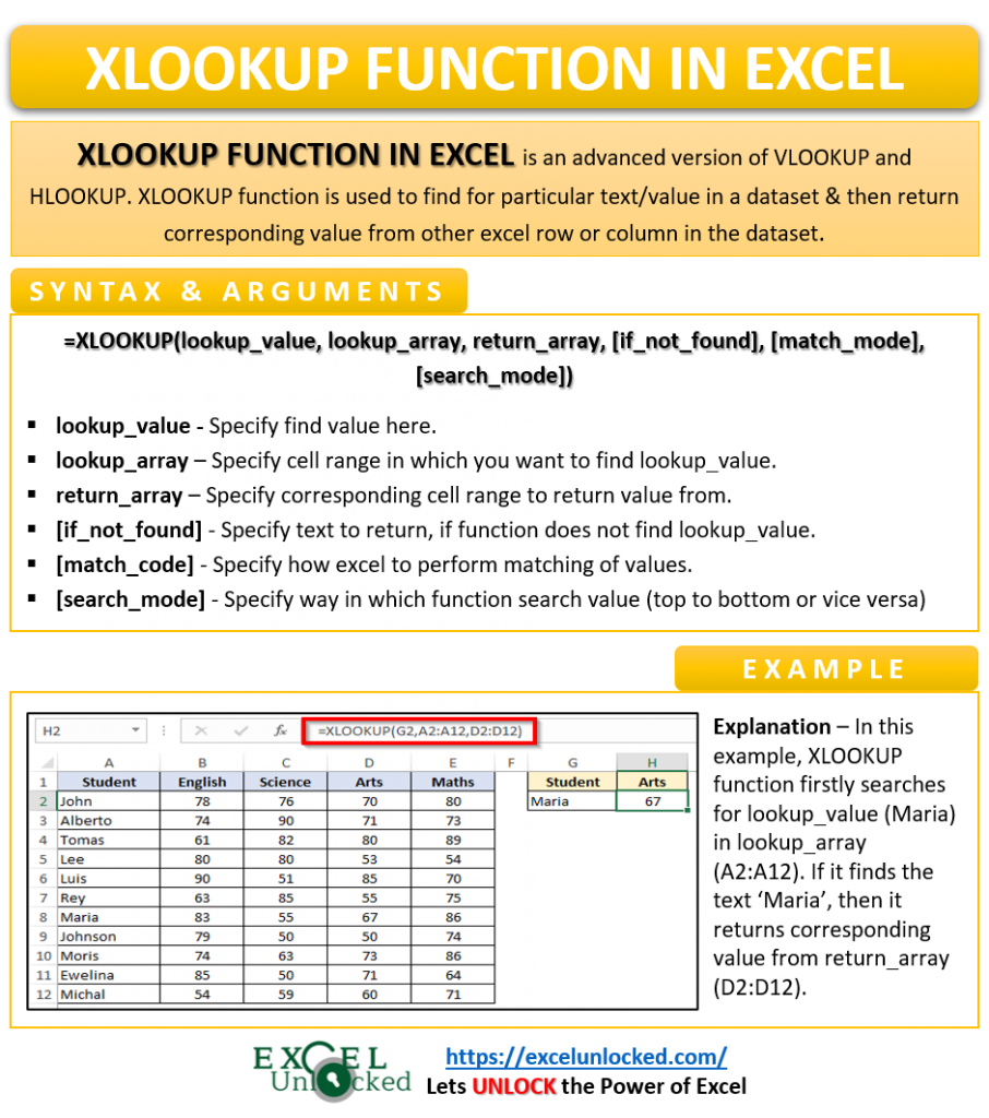
Let’s suppose you want to fetch the marks secured by ‘Maria’ in the subject ‘Arts’.

To do so, simply use the below formula:

=XLOOKUP(G2,A2:A12,D2:D12)

As a result, excel return the value as 67 (Marks obtained by Maria in Arts).

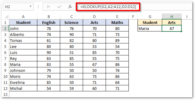
Explanation – In the above example, the XLOOKUP function firstly searches for lookup_value (Maria) in lookup_array (A2:A12). If it finds the lookup_value, then it returns corresponding value from the return_array (D2:D12).

Similarly, =XLOOKUP(“Moris”,A2:A12,E2:E12) would return marks obtained by Moris in Maths (viz. 87).

Note that since this is the first example, I have only made you understand the mandatory arguments of the XLOOKUP function. We would slowly get into the optional arguments as we go further through this blog.

Example # 2 – Return Text if Value Not Found in XLOOKUP

Suppose in the above example, the XLOOKUP function does not find the lookup_value in the lookup_array, then it returns #N/A formula error.

=XLOOKUP(“Mark”,A2:A12,E2:E12) returns #N/A error, because “Mark” is not in the list.

Interestingly, the XLOOKUP function can itself handle such errors. It means that if error occurs in XLOOKUP formula, then you can manage it within this formula.

This can be achieved by using the fourth argument of XLOOKUP function i.e. [if_not_found].

In the fourth argument, simply enter the text/value that you want to return within double-quotes, if XLOOKUP function gives error.

=XLOOKUP("Mark",A2:A12,E2:E12,"No Data")

Example # 3 – Fetch Entire Row Record Based on Lookup Value

Unlike the VLOOKUP function, which only allows you to get value from one particular column, the XLOOKUP formula has enhanced functionality.

Using excel XLOOKUP formula, you can fetch entire record corresponding to the lookup value.

To do so, simply select the entire record as return_array, as demonstrated below:

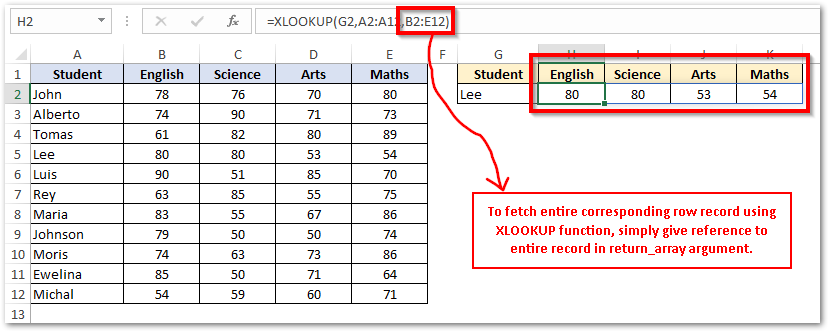
Note that in the above example, the XLOOKUP formula is only available in cell H2 and not in the other cells (I2, J2, and K2). The formula has automatically extended to the other cells I2, J2, and K2.

This means that you cannot directly delete the formula in automatically extended cells I2, J2, and K2. Instead, to delete the formula in all the cells, simply, select the original cell H2 and then press the ‘Delete’ key on your keyboard. This would remove the formula from all the cells (original cell + extended cells).

Example # 4 Using [match_code] in XLOOKUP Excel Function

The [match_code] argument is the fifth argument of the XLOOKUP function in excel which is useful to perform an approximate match of values.

This argument accepts following four values:

• 0 – This is a default value of XLOOKUP function. In this, the XLOOKUP formula searches for an exact match of lookup_value in the lookup_array and based on the matching, returns the result. (already learned in the above examples)

• -1 – It fetches the next smallest value if there is no exact matching of values in excel.

• 1 – It returns the next largest value if there is no exact matching of values in excel.

• 2 – Use argument value as 2 if you want to perform a partial match of values using wildcard characters (* and ?) in excel. (to be learned in upcoming section)

Let’s take one example to understand this in more detail.

The below image contains the sales values achieved by respective sales man and you want to find commission using the commission rate on the table to the right.

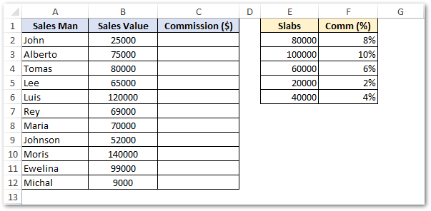
For finding the commission of each salesperson in excel, simply use the following formula in cell C2 and drag the formula to the other cells in column C, to get the sales commission for all the person.

=XLOOKUP(B2,$E$2:$E$6,$F$2:$F$6,,-1)*B2

As a result, you would get the commission value of 500. XLOOKUP function picks the commission rate as 5%.

Explanation – The XLOOKUP function first tries to find an exact match of lookup_value 25,000 in lookup_array (E2:E6). Since it does not find the exact match of value, the -1 match_code returns the return_value based on the next smallest value i.e. 20,000.

Unlike the VLOOKUP and HLOOKUP excel functions, there is no need to arrange the lookup_array in ascending or descending order for an approximate match of the value.

Example # 5 – Using Wildcard Characters in XLOOKUP Function

For me the wildcard characters (asterisk and question mark) are like a life-jacket.

The wildcard characters (* and ?) helps to search for a particular word/string in a cell instead of the entire cell content in excel.

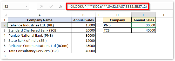
Let’s suppose you have names of companies along with its short name in column A. Column B contains the annual sales figures for the same.

Now, you want to get the annual sales of company based on the short name.

To achieve this, you can use the wildcard characters in the XLOOKUP function. However, for this, you need to specify the number ‘2’ in the fifth argument [match_code] of this function.

Enter below formula in cell E2:

=XLOOKUP("*"&D2&"*",$A$2:$A$7,$B$2:$B$7,,2)

Explanation – In the lookup_value “*”&D2&”*”, the * (asterisk symbol) is used before and after the lookup string D2 to find a particular word or string in a cell. In the above formula, the wildcard character (*) helps to search for the word ‘PNB’ in the entire cell content and if the search is successful, the XLOOKUP function returns the value from the lookup_array.

Check this link to know more about other wildcard characters in excel and its use.

Example # 6 – Using [search_mode] argument in XLOOKUP Excel Function

The [search_mode] argument is the sixth and the last argument of the XLOOKUP excel formula which denotes in which way should excel perform match of values.

It accepts below four values:

• 1 – This value specifies that excel should start matching the values from top to bottom (i.e. from the first value to the last value). This is the default search_mode if you keep the argument blank.

• -1 – This value acts exactly opposite to the above one. The search_mode -1 starts matching the values from bottom to top (i.e. from the last value to the first value).

• 2 – For this argument to work, it is must that the data is sorted in ascending order, otherwise formula may give error or a wrong result.

• -2 – For this argument to work, it is must that the data is sorted in descending order, otherwise formula may give error or a wrong result.

Example # 7 – Lookup from Right to Left in a Table

One of the limitation of using the VLOOKUP function in excel is that the VLOOKUP function can only lookup from left to right.

Also, the lookup value must be in the left-most cell range of lookup_array.

This drawback of VLOOKUP function has been eliminated by the introduction of XLOOKUP excel formula.

See the image below. The lookup_array is placed on the right of the return_array range.

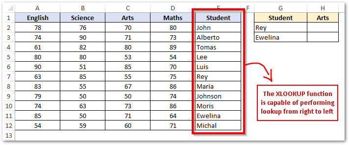
In this case, the formula in cell H2 will be:

=XLOOKUP(G2,$E$2:$E$12,$C$2:$C$12)

In the above examples, the lookup_array is $E$2:$E$12 and the return_array is $C$2:$C$12.

Therefore, using the XLOOKUP function you can return value from the column to the left of the lookup_array.

Thanks You 🙂