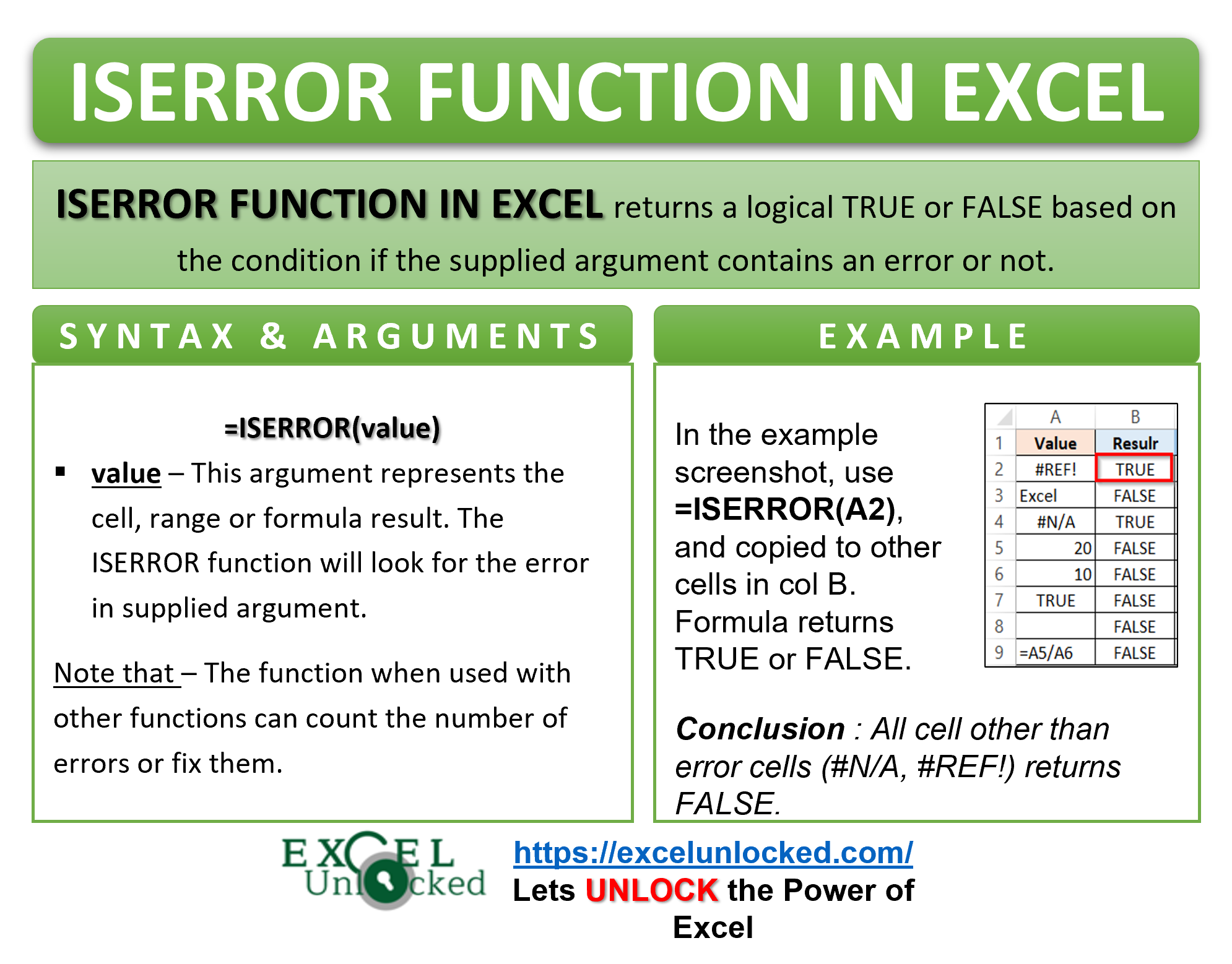
While working with the formulas in Excel, we may come across various kinds of excel formula errors. Therefore, we need to cope with these unwelcomed errors. Anything we can do to clean, count or represent those errors is by using the ISERROR Function of Excel. Let us see how.
Here we go 😎
When to Use ISERROR Function in Excel
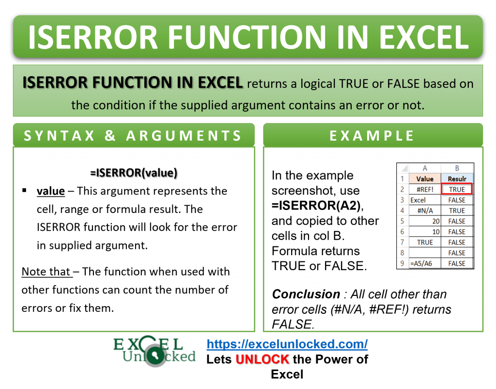
The expression ISERROR represents “is there any error in the cell?”. The ISERROR formula in excel helps us know if the passed argument contains an error or not. The function returns a boolean TRUE for the erroneous cells.
Whereas, if there are no errors (i.e. cells containing text strings, numbers, or formulas), the excel ISERROR formula returns FALSE.
We can use the function to count the number of error messages, present the errors in a clean way, or highlight the erroneous cells.
This function is categorized under the Information functions of Excel.
Syntax and Arguments
=ISERROR(value)
The below point explains the value argument of the ISERROR function of excel.
- value – In this argument, specify the cell, range or a formula result. The ISERROR function checks if the supplied argument contains or returns any error or not.
Points to Remember About Excel ISERROR Function
The following points must be kept in mind before the actual usage of the ISERROR Formula of excel.
- Unlike the ISERR function of Excel, the ISERROR formula returns a logical TRUE when the supplied argument containing #N/A error.
- An array is a collection of similar values. When we supply a range of cells to the ISERROR formula, it returns an array of boolean values (TRUE or FALSE) for all the cells in the range. Consequently, the formula will work as an array formula.
- We can use the ISERROR Formula with the SUM formula to get the total number of errors. (Refer to Example 2 in upcoming section).
- The ISERROR function when used with the IF formula, represent the error messages in a clean way. (refer example 3 in upcoming section).
Using Excel ISERROR Function with Examples
In this section of the blog, we will be doing some practical examples to learn the usage of the ISERROR formula in excel.
Ex. 1 – Simplest Example for ISERROR Function
Let us see how the ISERROR excel function works with different types of the value argument.
In the below image, column A contains a list of values.
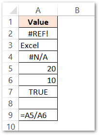
Use the following ISERROR Formula in cell B2 and copy it to other cells in column B.
=ISERROR(A2)
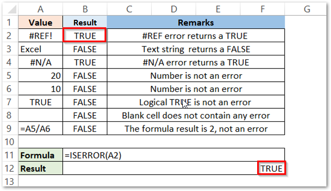
The Remarks column in the above image clearly explains the reason for the ISERROR function output.
Ex. 2 – Counting Total Number of Errors Using ISERROR with SUM Function
In this example, we will pass a range of cells to the ISERROR Function and then use the result to count the number of errors. Below is the required range of cells.

Enter the following formula in the target cell and then simply press Ctrl + Shift + Enter on your keyboard.
=SUM(--ISERROR(A1:F1))
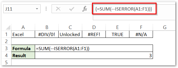
As a result, the formula returns the total number of errors to be 3.
Explanation – Let us see in steps how did the formula conclude this result.
- ISERROR function checked the error for the range A1:F1 and returned the result as an array {FALSE; TRUE; FALSE; TRUE; FALSE; TRUE}
- We applied the unary operator (–) to the array and converted the result to {0;1;0;1;0;1}. 0 for logical FALSE and 1 for logical TRUE.
- Finally, the SUM formula returned the sum of the array of elements 0+1+0+1+0+1=3.
When we press ctrl+shift+enter after typing the array formula, excel automatically adds curly brackets around the formula. You can also check the highlighted formula bar in the above example.
Ex. 3 – Cleaning Errors By Using IF function With ISERROR Function
While working with formulas in Excel, we might need to represent the results formally in a clean way. Instead of displaying the fussy error messages like #NUM!, #REF!, #DIV/0, we can give any other alternate text string.
Look at the below example. Here we have divided the values in column A with values in column B.
=A2/B2
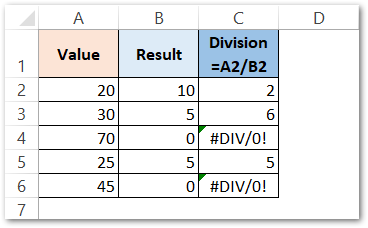
As a result, the formula performs division.
You will notice that the formula returned #DIV/0! error code in cells C4 and C6.
Use this formula to fix excel error messages.
=IF(ISERROR(A2/B2),"oops!",A2/B2)
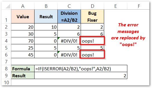
As a result, the formula returns the text string “oops!” instead of actual excel error message.
Explanation – The condition in the IF formula is ISERROR(A2/B2). If the division of A2 and B2 gives an error then the formula returns TRUE, otherwise, it returns FALSE (for no error). When the IF formula condition is TRUE, the function displays a text string “oops!”. If the condition is FALSE then the result will be A2/B2. The condition is TRUE for cells C4 and C6 (erroneous cells) thus the function returned a text string “oops!”.
This brings us to the end of the function blog!
Thank you for reading 😉
RELATED POSTS
- ISERR Function in Excel – Checking If The Cell Contains An Error
- ISNA Function in Excel – Checking for #N/A Errors
- ISREF Function in Excel – Checking for Cell Reference
- T Function in Excel – Usage with Examples
- ISLOGICAL Function in Excel – Checking for Boolean TRUE/FALSE
- 8 Errors in Formula in Excel and How to Resolve

