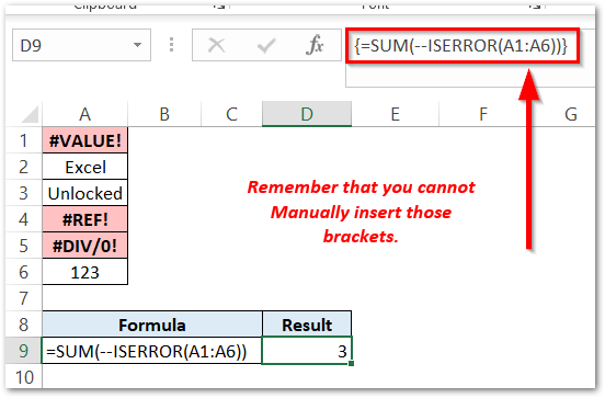
While working with the excel functions, you may encounter some or the other excel formula error, which we need to fix. There are two functions that would help you to deal with the errors – ISERROR and ISERR function in excel. These two formulas are very similar, with a very slight difference.
In this blog, we would learn how to use the ISERR formula in excel to deal with errors.
Here we go 😎
When To Use the Excel ISERR Function.
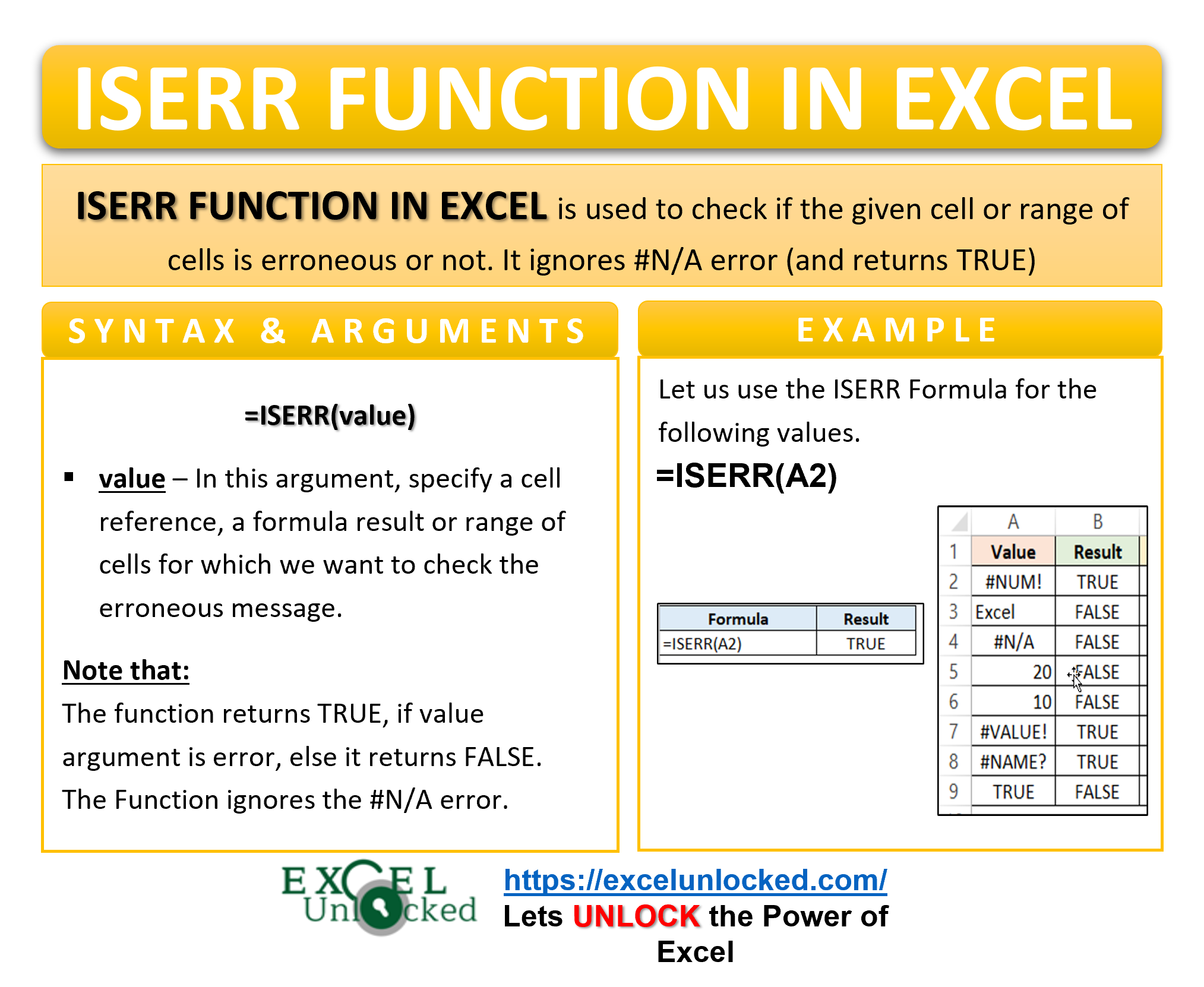
The ISERR Function returns a boolean (i.e. TRUE or FALSE) based on the supplied argument result. The function belongs to the Information function group.
It is important to note that the ISERR function does not work with #N/A errors. This is one of the major differences between the ISERR and ISERROR excel functions.
What Does ISERR Function Return?
- TRUE – The function returns TRUE when the function argument is an error like #NUM! , #NULL!, #NAME?, #VALUE!, #DIV/0! or #REF!.
- FALSE – The ISERR formula returns a FALSE for the #N/A error or any other not an error cell value.
Syntax and Arguments
=ISERR(value)
The below point explain the required function argument for ISERR Formula.
- value – In this argument, enter the cell reference, the result of a formula, or range of cells to check for the error.
Examples To Learn Usage of Excel ISERR Formula
In this section of the blog. we will perform some practical examples to learn the usage of the ISERR Function.
Ex. 1 – Simplest Example To Learn ISERR Function
In this example, we will try a variety of the ISERR function arguments and then check the result for each of them.
Below are the required function arguments.
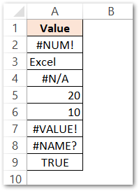
Use the following ISERR Formula to get the corresponding results.
=ISERR(A2)
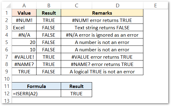
As a result, the formula returns TRUE for the first record. Use the excel fill handle tool to copy the formula to the rest of the cells.
Alternatively, you can also pass another formula inside the excel ISERR function, like this
=ISERR(A1/A2)
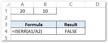
Explanation – We have passed the division of cell values in A1 and A2. A1/A2 gives 2 which further acts as a function argument for the ISERR Formula. Finally, the ISERR Formula returns a Logical FALSE because the number 2 is a non-erroneous value.
Ex. 2 – Counting the Number Of Errors Using the ISERR function with SUM Formula
In this example, let us say we want to count the number of error messages we have in the data.
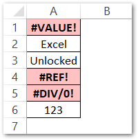
The red block indicates the error messages.
Enter the following formula and simply press Ctrl + Shift + Enter (CSE) to return the count the number of error messages.
=SUM(--ISERROR(A1:A6))
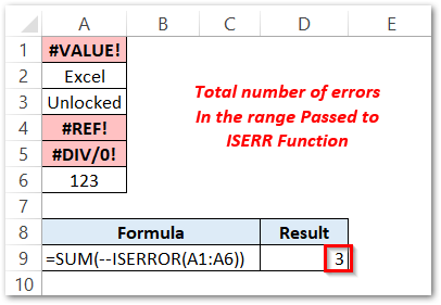
As a result, the formula has returned the total number of errors to be 3.
Explanation – The below bullet points explain each of the segments of the above formula:
- The ISERR(A1:A6) function returns the TRUE or FALSE for the range A1:A6. It returns the array of elements like this {TRUE; FALSE; FALSE; TRUE; TRUE; FALSE}
- The double minus before the ISERR function converts the array in to 1 and 0 (where, 1 represents TRUE, 0 represents FALSE) . The array of elements becomes {1;0;0;1;1;0}.
- After that the SUM function returns the sum of these array elements 1+0+0+1+1+0 which gives 3. This is the total number of errors in the array.
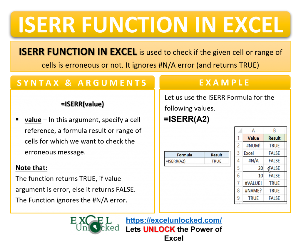
The formula we used above is an array formula. We need to press Ctrl + Shift + Enter (CSE Formula) to get the results. Pressing Ctrl+Shift+Enter inserts curly brackets around the formula. See the formula bar.
Ex. 3 – Using the ISERR Formula with the IF Function of Excel
The IF Function of Excel when used with the ISERR function fixes the erroneous messages we get while copying the formula for the rest of the cells.
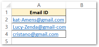
Let us say in this example, we have the customer email ids as follows.
Using the LEFT and FIND Combination
We want to extract the customer names from each of the email ids. For that, we are going to use the LEFT and FIND Functions of Excel. Below is the formula.
=LEFT(A2,FIND("-",A2,1)-1)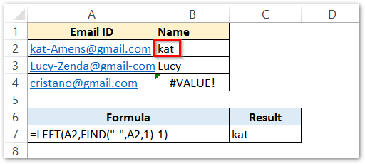
As a result, the function has extracted the name from the email id. We can copy the formula to the rest of the email ids.
Explanation – The LEFT Function is supplied with two arguments. text is cell A2. The num
_char ( number of characters we want to extract) is FIND(“-“,A2,1)-1. The FIND formula will find the “-” and return its position ( 4th position ) in cell A2. After that we subtract from it 1(3rd position) to get the text before “-“. The LEFT formula simply extracted the three characters from the left of cell A2 until it encounters “-“.
For the third email address, there is no “-” so the function returned a #VALUE! error because there is no hyphen in the email address contained in cell A4.
Cleaning the House!
What if instead of displaying an error message, we want the cell to be left blank. Use the following formula.
=IF(ISERR(LEFT(A2,FIND("-",A2,1)-1))," ",LEFT(A2,FIND("-",A2,1)-1))
As a result, when the formula is copied to cells C3 and C4 the cell does not show any error message.
Explanation – The condition of IF formula is ISERR(LEFT(A2,FIND(“-“,A2,1)-1)). If the result of the LEFT and FIND formula gives an error then the ISERR Function will return a TRUE or else FALSE. The IF function is applied such that if the result of the condition is TRUE ( error ) then the entire formula returns an empty string (” “). If the condition result of the IF formula is FALSE ( no error ) then the entire formula returns the result of the LEFT and FIND combination.
This brings us to the end of the ISERR Function blog.
Thank you for reading 😉
RELATED POSTS
- ISLOGICAL Function in Excel – Checking for Boolean TRUE/FALSE
- ERROR.TYPE Function in Excel – Error Codes,Examples
- ISREF Function in Excel – Checking for Cell Reference
- ISNA Function in Excel – Checking for #N/A Errors
- ISNUMBER Function of Excel – Checking If Cell Contains a Number
- T Function in Excel – Usage with Examples

