In a previous blog, we had learned how to extract the text from the left of a string with the help of excel’s LEFT function. Likewise, the RIGHT function in excel is used to extract a certain number of characters from the right of a string or text.
In this article, we would unlock everything about the Excel RIGHT function along with simple to advanced examples.
Here we go 😎
When to Use RIGHT Function in Excel
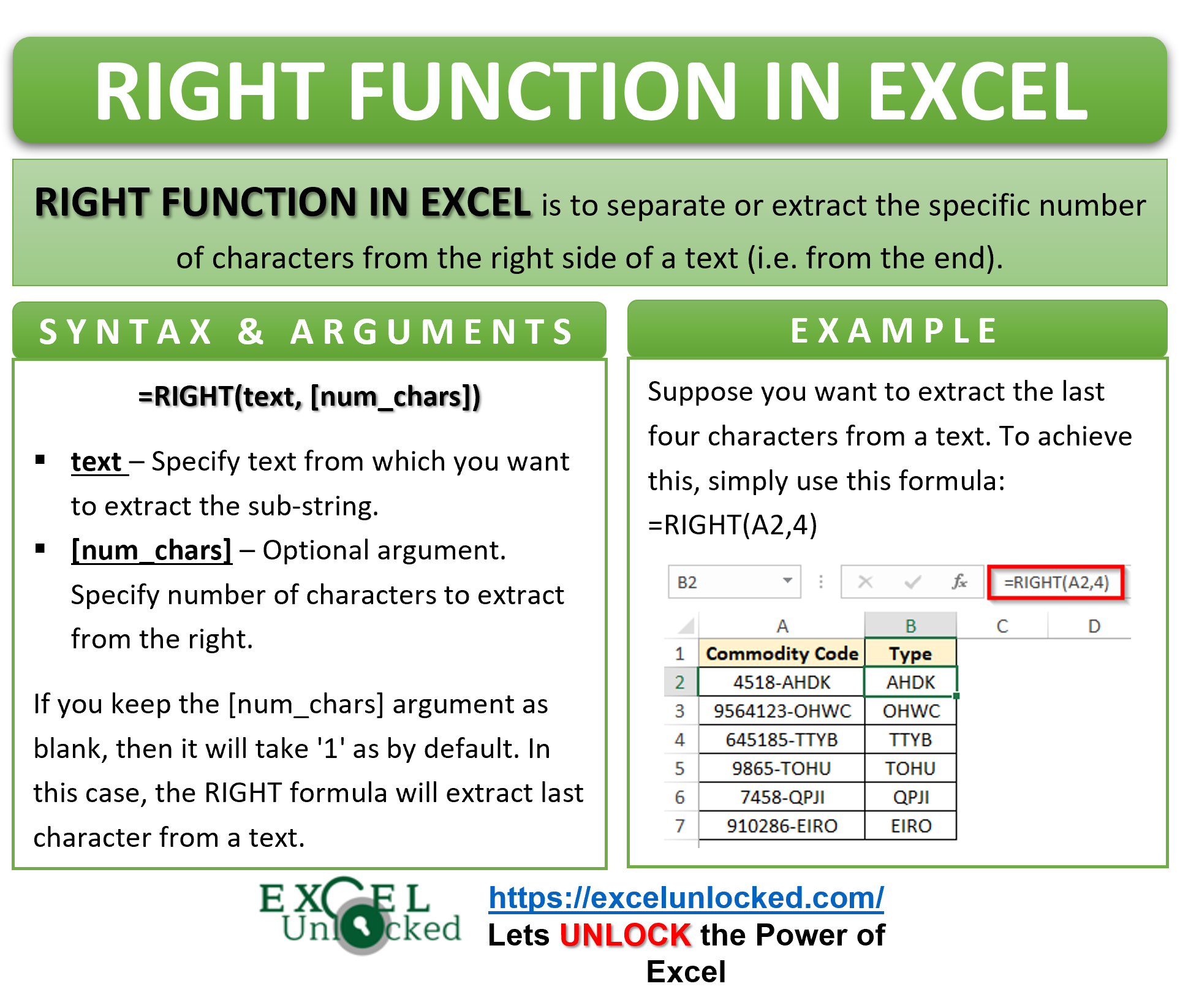
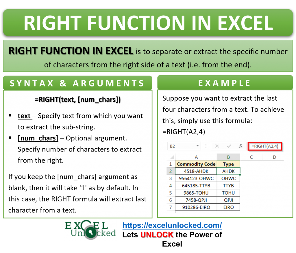
The excel RIGHT formula is used to get a specific number of characters from the end of a particular text string. The text string may be either manually entered in the formula or used as a cell reference.
Syntax and Arguments
=RIGHT(text, [num_chars])
The RIGHT function has two input arguments. The arguments are exactly the same as that of the LEFT function.
- text – In the text argument, enter the string (within double quotes) or the cell reference from which you want to extract the text.
- [num_chars] – In this argument, specify the number of characters that you want to extract.
Since the [num_chars] argument is optional, you may leave it blank. A blank [num_chars] argument defaults 1 which means the formula will extract the last character from the text string.
Examples of Excel RIGHT Function
Let us now see some examples from basic to advanced and understand how does the RIGHT function work in excel.
Ex. 1 # Extract Last Character from a Text or Cell in Excel
The below image shows the list of commodity codes where in the last character represents the commodity type.
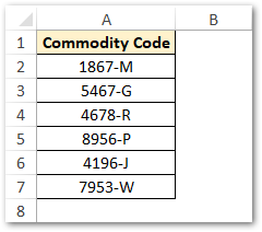
Now, suppose you want to extract the one character from the end (i.e. the commodity type letter).
You can achieve this by either using the Excel Text to Column functionality (Fixed Length Delimiter) or the RIGHT formula in excel.
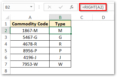
Simply use any of the following formulas:
=RIGHT(A2)
OR
=RIGHT(A2,1)
As a result, excel returns the last characters, as shown in the image below:
Ex. 2 # Extract Specific Number of Characters from End of Text String
To extract a particular number of characters from the right of the text or cell, use the [num_chars] argument.
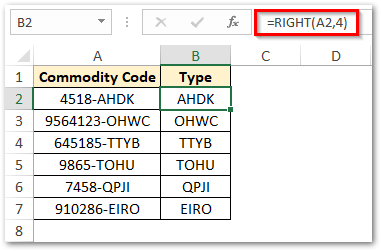
In the above examples, we have used the following formula to extract four characters from the right of the texts in column A.
=RIGHT(A2,4)
Ex. 3 # Extract All Text After a Particular Text or Symbol
In Ex. 2 above, the [num_chars] was constant (i.e. 4) in each of the values in column A. Therefore, simply putting 4 as [num_chars] value was enough to achieve the desired output.
However, in many practical situations, the exact number of characters to be extracted from the end is not constant.
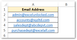
For example, in the below image the length of the domain (i.e. string after @ symbol) in the email addresses is different in each cell. Therefore, using a constant value in the [num_chars] argument will not work.
To create dynamic [num_chars] value, use the following formula:
=RIGHT(A2,LEN(A2)-FIND("@",A2))
OR
=RIGHT(A2,LEN(A2)-SEARCH("@",A2))
As a result, excel will extract and return the company name from the email address (i.e. extract values after @ symbol). See image below:
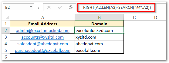
Explanation – The LEN(A2) function returns the total number of characters or letters in entire email address (cell A2). SEARCH and/or FIND function returns the position of the ‘@’ symbol. Finally, LEN(A2)-SEARCH(“@”,A2) will smartly return the position of ‘@’ from the right side of the email address. 😉
With this you may also be interested to learn about how to separate the first name from the full name in excel.
Thank You 🙂

